【Pre-processing Method】Various ways to visualize audio data
1. Waveform
Waveform is Most directly depiction of sound.
x-axis represent time, y-axis represent amplitude.
%time
import librosa
import librosa.display
import matplotlib.pyplot as plt

y, sr = librosa.load(librosa.ex('trumpet'))  # Load example audio
plt.figure(figsize=(10, 4))
librosa.display.waveshow(y, sr=sr)
plt.title('Waveform')
plt.xlabel('Time (s)')
plt.ylabel('Amplitude')
plt.show()
・Example

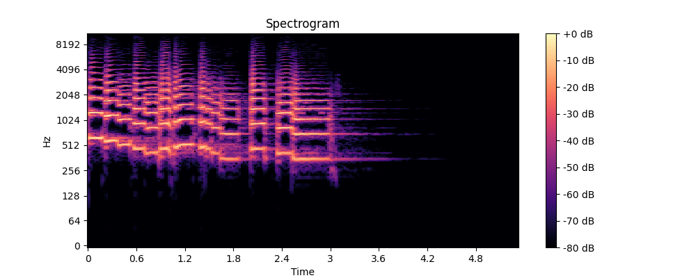
2. Spectrogram
Spectrogram is a visualization of frequency components by dividing waveform data by time and using Fourier transform.
It captures both time and frequency information, this very useful method is used in various scenes. however, depending on the size of the time window, some information may be lost on each side.
%time
import numpy as np

D = librosa.amplitude_to_db(np.abs(librosa.stft(y)), ref=np.max)
plt.figure(figsize=(10, 4))
librosa.display.specshow(D, sr=sr, x_axis='time', y_axis='log')
plt.colorbar(format='%+2.0f dB')
plt.title('Spectrogram')
plt.show()
・Example
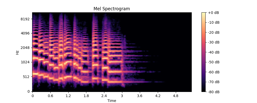
3. Mel spectrogram
Mel spectrogram is a type of spectrogram.
It is made easier to understand for huamns, and can be obtained by applying some processing after performing that to create normal spectrogam.
Simply put, it is an enhancement of the low frequency components of the spectrogram.
More details can be found here.
%time

S = librosa.feature.melspectrogram(y=y, sr=sr, n_mels=128)
S_DB = librosa.power_to_db(S, ref=np.max)
plt.figure(figsize=(10, 4))
librosa.display.specshow(S_DB, sr=sr, x_axis='time', y_axis='mel')
plt.colorbar(format='%+2.0f dB')
plt.title('Mel Spectrogram')
plt.show()
・Example
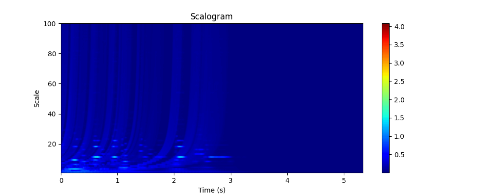
4. Scalogram
Scalogram is result of applying CWT(Continuing Wavelet Transform).
It provide frequency representation fewer loss than spectrogram with time direction.
More details can be found here.
%time
import pywt

scales = pywt.central_frequency('cmor') / np.linspace(1, 100, 100) * sr
cwtmatr, freqs = pywt.cwt(y, scales, 'cmor', sampling_period=1/sr)
plt.figure(figsize=(10, 4))
plt.imshow(abs(cwtmatr), aspect='auto', extent=[0, len(y) / sr, 1, 100], cmap='jet', origin='lower')
plt.colorbar()
plt.title('Scalogram')
plt.xlabel('Time (s)')
plt.ylabel('Scale')
plt.show()
・Example
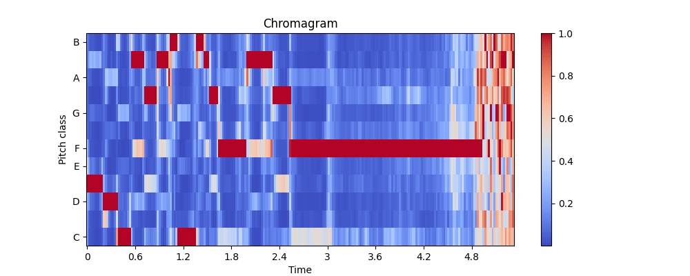
5. Chromagram
Chromagram provides 'rougth' freqency information.
It is obtained by this formula.
More details can be found here.
%time

C = librosa.feature.chroma_cqt(y=y, sr=sr)
plt.figure(figsize=(10, 4))
librosa.display.specshow(C, sr=sr, x_axis='time', y_axis='chroma', cmap='coolwarm')
plt.colorbar()
plt.title('Chromagram')
plt.show()
・Example
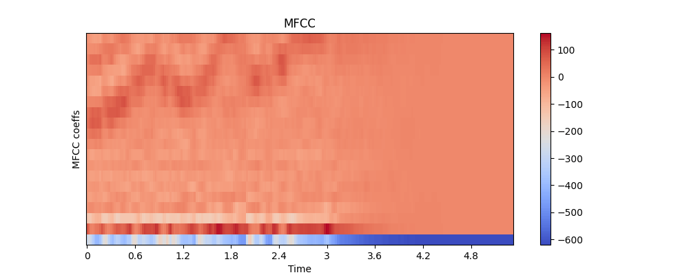
6. Mel-Frequency Cepstral Coefficients (MFCCs)
MFCCs quantity the self-similarity of the high-pass filtered signal at different time scales (musical pitch removed, robust to bandwidth reduction).
It is useful for analysis of the human voice data, etc.
More details can be found here
%time

mfccs = librosa.feature.mfcc(y=y, sr=sr)
plt.figure(figsize=(10, 4))
librosa.display.specshow(mfccs, sr=sr, x_axis='time')
plt.ylabel('MFCC coeffs')
plt.colorbar()
plt.title('MFCC')
plt.show()
・Example
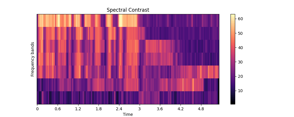
7. Spectral Contrast
Spectral Contrast shows intensity of change in specified frequency range in each time window. It helps recognition of music genre, texture, complexity or more details audio.
More details can be found here
%time

contrast = librosa.feature.spectral_contrast(y=y, sr=sr)
plt.figure(figsize=(10, 4))
librosa.display.specshow(contrast, x_axis='time')
plt.colorbar()
plt.ylabel('Frequency bands')
plt.title('Spectral Contrast')
plt.show()
・Example
Summary
In this time, I summarized some way to visualize wave data.
I'm glad this article will be helpful to someone.
Discussion