🎄
LightGBM vs XGBoostを比較してみた
📌はじめに
以前LightGBMって本当に強い?決定木と比べて検証してみたを投稿しましたが、
やっぱり気になるのは LightGBM vs XGBoost ですよね。
「結局どっちが強いの?」
「精度に差はあるの?」
そこで今回は、LightGBM vs XGBoost を同じ条件で比較し、
その違いを確かめてみたいと思います。
❓LightGBM vs XGBoost の違いって❓
📌共通点
- ブースティング木モデル(弱学習器=決定木を多数積み重ねる)
- 回帰・分類・ランキングなど幅広いタスクに対応
- 欠損値処理や正則化を組み込み
- GPU対応あり
📌主な違い
1. 木の成長方式
-
XGBoost:深さ優先で木を伸ばす(level-wise growth)
- 同じ深さのノードを一気に分割
- バランスの良い木を作りやすい
- 計算量は増えるが、安定性が高い
-
LightGBM:リーフごとに分割を進める(leaf-wise growth)
- 損失減少が最大になる葉を優先して分割
- 精度が高くなりやすい
- ただし過学習しやすい(深い木になりがち)
2. 特徴量の扱い
- XGBoost:全特徴量を対象に分割候補を探索
-
LightGBM:
- Gradient-based One-Side Sampling (GOSS) → 勾配の大きいサンプルを優先的に使う
- Exclusive Feature Bundling (EFB) → 疎な特徴量をまとめて効率化
👉 高次元・大規模データに強いのは LightGBM。
3. メモリ・速度
- LightGBM:メモリ効率が高く、学習が速い(大規模データ向き)
- XGBoost:少し重めだが、安定性とチューニングのしやすさが強み
4. ハイパーパラメータの傾向
-
XGBoost:やや直感的(
max_depth,etaなど) -
LightGBM:パラメータが独特で学習コントロールに慣れが必要(
num_leaves,max_depthの関係など)
✅まとめ
- データが大きい/特徴量が多い/速度重視 → LightGBM
- 安定性/細かい制御/チューニングしやすさ重視 → XGBoost
📌サンプルデータ:sample_car_data.csv
機械学習モデルの予測根拠を可視化:LightGBM × SHAP入門でも使用した

sample_car_data.csv(N = 400)
📌LightGBMデータ:predictions_with_top3.csv
XGBoostとの比較に使用
機械学習モデルの予測根拠を可視化:LightGBM × SHAP入門で作成した

predictions_with_top3.csv
📌フォルダ構成
├─ 1_flow/
│   └─ shap_analysis_xgboost.py     # 実行スクリプト
├─ 2_data/
│   │─ sample_car_data.csv          # サンプルデータ
│   └─ predictions_with_top3.csv    # XGBoostとの比較に使用するデータ
├─ 3_output/                        # 出力用(自動作成)
📌環境
python3.x
📌コード(shap_analysis_xgboost.py)
コード:ライブラリ~sample_car_data.csv読み込み
#============================================
# ライブラリと変数設定
#============================================
import os
import shap
import sys
import numpy as np
import pandas as pd
import matplotlib.pyplot as plt
from sklearn.model_selection import train_test_split
from sklearn.preprocessing import LabelEncoder
from sklearn.metrics import accuracy_score, f1_score, ConfusionMatrixDisplay
from sklearn.tree import DecisionTreeClassifier, plot_tree
import lightgbm as lgb
import japanize_matplotlib
from xgboost import plot_importance
from xgboost import XGBClassifier, plot_tree as xgb_plot_tree
import xgboost as xgb


INPUT_FOLDER = '2_data'
INPUT_FILE = 'sample_car_data.csv'
INPUT_TOP3_FILE = "predictions_with_top3.csv"
OUTPUT_FOLDER = '3_output'

ID = 'customer_id'
target_col = 'manufacturer'
numeric_cols = ["family", "age", "children", "income"]

# 結合時にリネームする
re_name_be = "predicted_manufacturer"
re_name_af =  "predicted_class"

# =========================
# ディレクトリ・ファイル設定
# =========================
parent_path = os.path.dirname(os.getcwd())
input_path = os.path.join(parent_path, INPUT_FOLDER, INPUT_FILE)
input_top3_path = os.path.join(parent_path, INPUT_FOLDER, INPUT_TOP3_FILE)
output_path = os.path.join(parent_path, OUTPUT_FOLDER)
os.makedirs(output_path, exist_ok=True)

save_tree3models_path = os.path.join(output_path, "Confusion_Matrix_3models.png")
save_Feature_path  = os.path.join(output_path, "比較_LightGBM_XGBoost_Feature.png")
save_path  = os.path.join(output_path, "predictions_with_top3_XGBoost.csv")
save_name_path  = os.path.join(output_path, "メーカー別_SHAP_特徴ランキングXGBoost.csv")


# =========================
# CSV読み込み
# =========================
try:
    df = pd.read_csv(input_path, encoding="utf-8")
except UnicodeDecodeError:
    df = pd.read_csv(input_path, encoding="cp932")
コード:カテゴリ列自動判定~混同行列
# =========================
# カテゴリ列自動判定
# =========================
exclude_cols = [ID, target_col]
categorical_cols = [col for col in df.columns if col not in exclude_cols + numeric_cols]
df[categorical_cols] = df[categorical_cols].astype("category")

# =========================
# 説明変数と目的変数
# =========================
X_df = df.drop([ID, target_col], axis=1)
y_df = df[target_col]

# クラス数を確認
classes = np.unique(y_df)
print("クラス:", classes)

# =========================
# ラベルを0始まりに変換(LightGBM対応)
# =========================
le = LabelEncoder()
y_enc = le.fit_transform(y_df)
class_names = [str(c) for c in le.classes_]

print("クラス:", class_names)

# =========================
# データ分割(test_size=0.25)
# =========================
X_train, X_test, y_train, y_test = train_test_split(
    X_df, y_enc, test_size=0.25, random_state=0, stratify=y_enc
)
print("訓練データ数:", len(X_train))
print("テストデータ数:", len(X_test))


# ======================================
# LightGBMモデル(訓練データのみで学習)
# ======================================
objective = 'binary' if len(class_names) == 2 else 'multiclass'
metric = 'binary_error' if objective == 'binary' else 'multi_error'
params = {'objective': objective, 'metric': metric, 'verbose': -1}
if objective == 'multiclass':
    params['num_class'] = len(class_names)

lgb_train = lgb.Dataset(X_train, label=y_train, feature_name=X_df.columns.tolist())
lgb_model = lgb.train(params, lgb_train, num_boost_round=50)
# 予測
y_pred_lgb_prob = lgb_model.predict(X_test)
# y_pred_lgb = (y_pred_lgb_prob > 0.5).astype(int) if objective=='binary' else np.argmax(y_pred_lgb_prob, axis=1)
if objective == 'binary':
    y_pred_lgb = (y_pred_lgb_prob > 0.5).astype(int)
else:
    y_pred_lgb = np.argmax(y_pred_lgb_prob, axis=1)

# ==================================
# XGBoostモデル(訓練/テスト分割で学習)
# ==================================
xgb_model = XGBClassifier(
    objective='multi:softmax' if len(class_names) > 2 else 'binary:logistic',
    num_class=len(class_names) if len(class_names) > 2 else None,
    eval_metric='mlogloss' if len(class_names) > 2 else 'logloss',
    use_label_encoder=False,
    random_state=42
)

X_train_enc = X_train.copy()
X_test_enc  = X_test.copy()

for col in X_train_enc.select_dtypes(include='category'):
    X_train_enc[col] = X_train_enc[col].cat.codes
    X_test_enc[col]  = X_test_enc[col].cat.codes

xgb_model.fit(X_train_enc, y_train)
y_pred_xgb = xgb_model.predict(X_test_enc)

# =========================
# 参考指標
# =========================
print("【LightGBM】     Accuracy:", accuracy_score(y_test, y_pred_lgb))
print("【LightGBM】     F1 Score:", f1_score(y_test, y_pred_lgb, average='weighted'))

print("【XGBoost】     Accuracy:", accuracy_score(y_test, y_pred_xgb))
print("【XGBoost】     F1 Score:", f1_score(y_test, y_pred_xgb, average='weighted'))

# =========================
# 混同行列
# =========================
fig, ax = plt.subplots(1, 2, figsize=(12,5))  #LGB / XGB
ConfusionMatrixDisplay.from_predictions(y_test, y_pred_lgb, ax=ax[0])
ax[0].set_title("LightGBM")
ConfusionMatrixDisplay.from_predictions(y_test, y_pred_xgb, ax=ax[1])
ax[1].set_title("XGBoost")

plt.tight_layout()
plt.savefig(save_tree3models_path, dpi=300)
plt.show()
出力例
【LightGBM】     Accuracy: 0.73
【LightGBM】     F1 Score: 0.7273653962492439
【XGBoost】     Accuracy: 0.72
【XGBoost】     F1 Score: 0.7213349682198088

❓精度向上:モデルのチューニング❓
今回の比較では、LightGBM と XGBoost を デフォルト設定 のまま使用しました。
デフォルト設定でも十分な性能が出る場合もありますが、
モデルの性能はハイパーパラメータによって大きく変わるためチューニングはとても重要です。
主なハイパーパラメータ
- n_estimators:学習する木の数
- max_depth:木の深さ
- learning_rate:学習率
- subsample / colsample_bytree:データや特徴量のサンプリング割合
- reg_alpha / reg_lambda:正則化パラメータ
チューニング方法
- GridSearchCV や RandomizedSearchCV を使って最適な組み合わせを探索
- データセットの特性や目的に応じて、Top-1 / Top-3 精度や F1 スコアを評価指標に設定
コード:木~集計(平均・最大・最小)
import json
from xgboost import plot_tree as xgb_plot_tree
from xgboost import XGBClassifier, plot_tree as xgb_plot_tree

# =========================
# LightGBM(1本目の木を可視化)
# =========================
plt.figure(figsize=(20, 10))
lgb.plot_tree(lgb_model, tree_index=0, figsize=(20,10), show_info=['split_gain', 'internal_value', 'internal_count', 'leaf_count'])
plt.title("LightGBM Tree (Tree 0)")
plt.savefig(os.path.join(output_path, "LightGBM_Tree.png"), dpi=300)
plt.show()


# =========================
# XGBoost(全データで学習、可視化用)
# =========================

# 全データをコピーしてカテゴリ列を整数化
X_df_enc = X_df.copy()
for col in X_df_enc.select_dtypes(include='category'):
    X_df_enc[col] = X_df_enc[col].cat.codes

# XGBoost 全データ学習(可視化用)
xgb_model_all = XGBClassifier(
    objective='multi:softmax' if len(class_names) > 2 else 'binary:logistic',
    num_class=len(class_names) if len(class_names) > 2 else None,
    eval_metric='mlogloss' if len(class_names) > 2 else 'logloss',
    use_label_encoder=False,
    random_state=42
)
xgb_model_all.fit(X_df_enc, y_enc)

# =========================
# XGBoost(1本目の木を可視化)
# =========================

plt.figure(figsize=(20, 10))
xgb_plot_tree(xgb_model_all, num_trees=0, rankdir='LR')
plt.title("XGBoost Tree (Tree 0)")
plt.savefig(os.path.join(output_path, "XGBoost_Tree.png"), dpi=300)
plt.show()

# =========================
# XGBoost 木の深さ・ノード数
# =========================
booster = xgb_model_all.get_booster()
trees_json = booster.get_dump(dump_format='json')

def get_depth(node):
    if "children" not in node or len(node["children"]) == 0:
        return 1
    return 1 + max(get_depth(child) for child in node["children"])

def count_nodes(node):
    if "children" not in node or len(node["children"]) == 0:
        return 1
    return 1 + sum(count_nodes(child) for child in node["children"])

xgb_tree_stats = []
for i, t_str in enumerate(trees_json):
    t = json.loads(t_str)
    depth = get_depth(t)
    nodes = count_nodes(t)
    xgb_tree_stats.append({"Tree": i, "Depth": depth, "Nodes": nodes})

xgb_stats_df = pd.DataFrame(xgb_tree_stats)

# =========================
# LightGBM 木の深さ・ノード数
# =========================
lgb_json = lgb_model.dump_model()

def get_depth_lgb(node):
    if "left_child" not in node and "right_child" not in node:
        return 1
    return 1 + max(get_depth_lgb(node["left_child"]), get_depth_lgb(node["right_child"]))

def count_nodes_lgb(node):
    if "left_child" not in node and "right_child" not in node:
        return 1
    return 1 + count_nodes_lgb(node["left_child"]) + count_nodes_lgb(node["right_child"])

lgb_tree_stats = []
for t, info in enumerate(lgb_json["tree_info"]):
    tree_t = info["tree_structure"]
    depth = get_depth_lgb(tree_t)
    nodes = count_nodes_lgb(tree_t)
    lgb_tree_stats.append({"Tree": t, "Depth": depth, "Nodes": nodes})

lgb_stats_df = pd.DataFrame(lgb_tree_stats)

# =========================
# 集計(平均・最大・最小)
# =========================
summary_df = pd.DataFrame({
    "Model": ["XGBoost", "LightGBM"],
    "Avg Depth": [xgb_stats_df["Depth"].mean(), lgb_stats_df["Depth"].mean()],
    "Max Depth": [xgb_stats_df["Depth"].max(), lgb_stats_df["Depth"].max()],
    "Min Depth": [xgb_stats_df["Depth"].min(), lgb_stats_df["Depth"].min()],
    "Avg Nodes": [xgb_stats_df["Nodes"].mean(), lgb_stats_df["Nodes"].mean()],
    "Max Nodes": [xgb_stats_df["Nodes"].max(), lgb_stats_df["Nodes"].max()],
    "Min Nodes": [xgb_stats_df["Nodes"].min(), lgb_stats_df["Nodes"].min()],
})

print("=== Tree Structure Summary ===")
print(summary_df)
出力例:全木を集計した統計値
=== Tree Structure Summary ===
      Model  Avg Depth  Max Depth  Min Depth  Avg Nodes  Max Nodes  Min Nodes
0   XGBoost   3.574286          7          1  10.562857         65          1
1  LightGBM   7.822857         11          3  23.611429         33          5
木 可視化
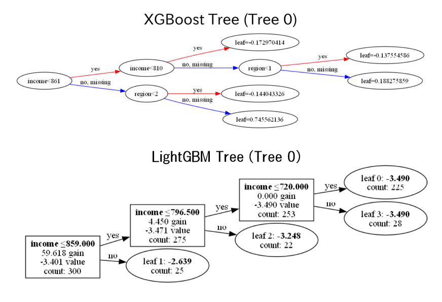
❓なぜ(Tree 0)なの❓
「0 番目の木を描いてますよ」 と言う意味です。
理由
- XGBoost や LightGBM は、複数本の木の集合(勾配ブースティング木)で構成される
- 学習後のモデルは「木が100本(num_boost_round=100)」のように多数ある
-
num_trees=0→ 最初の木(0 番目)を描画 -
num_trees=1→ 1 番目の木(2本目)を描画
補足
- 表の Avg Depth / Max Depth / Min Depth は 全木を集計した統計値
- 可視化は重いため、代表として Tree 0 だけを表示することが多い
コード:特徴量重要度~可視化
# ======================================
# LightGBM Feature Importance
# ======================================
lgb_imp = pd.DataFrame({
    "特徴量": lgb_model.feature_name(),
    "重要度": lgb_model.feature_importance()
}).sort_values("重要度", ascending=False)
lgb_imp.rename(columns={"重要度":"LightGBM"}, inplace=True)

# ======================================
# XGBoost Feature Importance
# ======================================
xgb_imp = pd.Series(xgb_model.get_booster().get_score(importance_type="weight")).sort_values(ascending=False)
xgb_imp = xgb_imp.reset_index()
xgb_imp.columns = ["特徴量","XGBoost"]

# ======================================
# 両方を結合して比較
# ======================================
feature_compare = pd.merge(lgb_imp, xgb_imp, on="特徴量", how="outer").fillna(0)
feature_compare = feature_compare.sort_values("XGBoost", ascending=False)
shap_compare_norm = feature_compare.copy()

shap_compare_norm["LightGBM"] = shap_compare_norm["LightGBM"] / shap_compare_norm["LightGBM"].max()
shap_compare_norm["XGBoost"]  = shap_compare_norm["XGBoost"]  / shap_compare_norm["XGBoost"].max()

print("=== Normalized Feature Importance Comparison ===")
print(shap_compare_norm.sort_values("XGBoost", ascending=False).head(10))

# ======================================
#  正規化 (0~1)
# ======================================
feature_compare_norm = feature_compare.copy()
feature_compare_norm["LightGBM"] = feature_compare_norm["LightGBM"] / feature_compare_norm["LightGBM"].max()
feature_compare_norm["XGBoost"] = feature_compare_norm["XGBoost"] / feature_compare_norm["XGBoost"].max()

# ======================================
# 上位 N 特徴量を XGBoost 順に取得(上位10特徴量)
# ======================================
topN = 10
top_features = feature_compare_norm.sort_values("XGBoost", ascending=False)["特徴量"].head(topN).values
light_values = feature_compare_norm.set_index("特徴量").loc[top_features, "LightGBM"].values
xgb_values = feature_compare_norm.set_index("特徴量").loc[top_features, "XGBoost"].values

# ======================================
# 可視化
# ======================================
x = np.arange(topN)
width = 0.35

fig, ax = plt.subplots(figsize=(10,6))
ax.barh(x - width/2, light_values[::-1], width, label="LightGBM", color="salmon")
ax.barh(x + width/2, xgb_values[::-1], width, label="XGBoost", color="skyblue")

ax.set_yticks(x)
ax.set_yticklabels(top_features[::-1])
ax.set_xlabel("Normalized Feature Importance")
ax.set_title("Normalized Feature Importance Comparison (Top 10)")
ax.legend()

# 棒上に数値表示
for i in range(topN):
    ax.text(light_values[::-1][i]+0.02, x[i]-width/2, f"{light_values[::-1][i]:.2f}", va='center')
    ax.text(xgb_values[::-1][i]+0.02, x[i]+width/2, f"{xgb_values[::-1][i]:.2f}", va='center')

plt.tight_layout()
plt.show()
出力例
=== Normalized Feature Importance Comparison ===
                     特徴量   XGBoost  LightGBM
0                 income  1.000000  1.000000
1                    age  0.746955  0.626979
2  previous_manufacturer  0.434371  0.045598
3                  hobby  0.345061  0.024699
4         car_preference  0.254398  0.031666
5                 family  0.230041  0.183661
6                 region  0.223275  0.210893
7               children  0.133965  0.112730
8                 gender  0.131258  0.105130
9        employment_type  0.085250  0.095630

コード:モデル定義~Top-3 Accuracy 計算
# ======================================
# モデル定義
# ======================================

xgb_model = xgb.XGBClassifier(
    objective="multi:softprob",
    num_class=len(classes),
    n_estimators=100,
    use_label_encoder=False,
    eval_metric="mlogloss",
    enable_categorical=True,
    random_state=42
)

# 全データで学習
xgb_model.fit(X_df, y_enc)

# ==============================
# XGBoost パラメータ設定
# ==============================
params = {
    "objective": "multi:softprob",  # 確率出力
    "num_class": len(classes),
    "eval_metric": "mlogloss",
    "verbosity": 0,
}

# ==============================
# 学習(100回で学習)
# ==============================
# xgb_model はすでに xgb.XGBClassifier で定義済みとします
xgb_model.set_params(n_estimators=100)
xgb_model.fit(X_df, y_enc)  # 全データで学習(可視化や予測用)

# ==============================
# 全データに対する予測
# ==============================
y_all_pred_prob = xgb_model.predict_proba(X_df)  # 予測確率
y_all_pred = np.argmax(y_all_pred_prob, axis=1)  # 予測クラスラベル

# ==============================
# 上位3候補の抽出
# ==============================
top3_classes = np.argsort(y_all_pred_prob, axis=1)[:, ::-1][:, :3]
top3_probs   = np.sort(y_all_pred_prob, axis=1)[:, ::-1][:, :3]

# ==============================
# 元データに結果を追加
# ==============================
df["predicted_manufacturer"] = y_all_pred

# 各クラス確率
for i in range(y_all_pred_prob.shape[1]):
    df[f"prob_class_{i}"] = y_all_pred_prob[:, i]

# 上位3クラス
for i in range(3):
    df[f"top{i+1}_class"] = top3_classes[:, i]
    df[f"top{i+1}_prob"] = top3_probs[:, i]

# 確認
print(df[[
    target_col,
    "predicted_manufacturer",
    "top1_class", "top1_prob",
    "top2_class", "top2_prob",
    "top3_class", "top3_prob"
]].head())

# ==============================
# Top-3 Accuracy 計算
# ==============================
top3_accuracy = np.mean([
    y_true in top3 for y_true, top3 in zip(y_enc, top3_classes)
])
print(f"Top-3 Accuracy: {top3_accuracy:.3f}")
出力例
  predicted_manufacturer  manufacturer  top1_class  top1_prob  top2_class  \
0             5                       5           5   0.989131           6
1             6                       6           6   0.949702           5
2             6                       6           6   0.989858           5
3             2                       2           2   0.991235           5
4             6                       6           6   0.969265           5

   top2_prob  top3_class  top3_prob
0   0.005029           0   0.002892
1   0.046880           2   0.000909
2   0.007324           0   0.000870
3   0.004172           0   0.001390
4   0.026152           3   0.002293
Top-3 Accuracy: 1.000
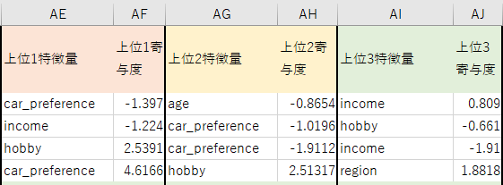
コード:XGBoostモデル SHAP値計算~XGBoost 上位3寄与特徴量抽出
# ==============================
# XGBoostモデル SHAP値計算
# ==============================

# X_df のコピーを作ってカテゴリ列を cat.codes に変換
X_df_enc = X_df.copy()
for col in X_df_enc.select_dtypes(include='category'):
    X_df_enc[col] = X_df_enc[col].cat.codes

# SHAP explainer & shap値計算
xgb_explainer = shap.TreeExplainer(xgb_model)

# ✅ ここは X_df_enc を渡す!
shap_xgb_values = xgb_explainer.shap_values(X_df_enc)


if isinstance(shap_xgb_values, list):
    # マルチクラス分類の場合
    print("SHAP values shape per class:", [v.shape for v in shap_xgb_values])
else:
    # バイナリ or 回帰の場合
    print("SHAP values shape:", shap_xgb_values.shap
# =======================================
# 正解が top3 の何番目だったかを記録(XGBoost版)
# =======================================
def top_rank_xgb(row):
    true_class = row[target_col]
    top_classes = [row["top1_class"], row["top2_class"], row["top3_class"]]
    return top_classes.index(true_class) + 1 if true_class in top_classes else None

df["correct_rank"] = df.apply(top_rank_xgb, axis=1)

# 結果を確認
print(df["correct_rank"].value_counts())

# ======================================
# XGBoost 上位3寄与特徴量抽出
# ======================================

# 学習済みモデル: xgb_model
# 学習に使った特徴量: X_df (DataFrame)

# TreeExplainer の作成
explainer = shap.TreeExplainer(xgb_model)

# shap_values を計算
shap_values = explainer(X_df)  # ← これで shap_values が Explanation オブジェクトに入る


results_top3 = []

# shap_values は explainer(X_df) の結果(Explanationオブジェクト)
# multi-class の場合 shap_values.values は (n_samples, n_classes, n_features)
# binary の場合は (n_samples, n_features)

for i in range(len(df)):
    pred_class = df.loc[i, re_name_be]

    # multi-class なら、pred_class に対応する行を取得
    if len(class_names) > 2:  # multi-class
        shap_vals = shap_values.values[i, pred_class, :]
    else:  # binary
        shap_vals = shap_values.values[i, :]

    features = list(X_df.columns)

    # 絶対値で上位3特徴量を選択
    top_idx = np.argsort(np.abs(shap_vals))[::-1][:3]
    top_features = [features[j] for j in top_idx]
    top_values = [shap_vals[j] for j in top_idx]

    tmp = {
        ID: df.loc[i, ID],
        re_name_af: pred_class,
        "top1_feature": top_features[0],
        "top1_value": top_values[0],
        "top2_feature": top_features[1],
        "top2_value": top_values[1],
        "top3_feature": top_features[2],
        "top3_value": top_values[2]
    }
    results_top3.append(tmp)

top3_df = pd.DataFrame(results_top3)
top3_df.head()
コード:結合準備~predictions_with_top3_XGBoost.csv出力
# ==============================
# 結合準備
# ==============================
# すでに top3_df では "predicted_manufacturer" を使っているので、元データ df も揃える
#df = df.rename(columns={re_name_be: "predicted_manufacturer"})
# 列名を統一
df = df.rename(columns={"predicted_manufacturer": re_name_af})

# CSV出力(UTF-8 BOM付き)
df.to_csv("チェック用_XGBoost.csv", index=False, encoding="utf-8-sig")

# ==============================
# マージ(ID と予測クラス列で結合)
# ==============================
df_merged = pd.merge(df, top3_df, on=[ID, re_name_af], how="left")

# ==============================
# 列名リネーム(必要に応じて追加)
# ==============================
rename_dict = {
    "customer_id": "顧客ID",
    "family": "同居家族",
    "age": "年齢",
    "gender": "性別",
    "income": "世帯収入",
    "marital_status": "婚姻状況",
    "region": "居住地",
    "employment_type": "雇用形態",
    "hobby": "趣味",
    "car_preference": "好みのボディタイプ",
    "previous_car_owner": "保有歴",
    "top1_feature": "上位1特徴量",
    "top1_value": "上位1寄与度",
    "top2_feature": "上位2特徴量",
    "top2_value": "上位2寄与度",
    "top3_feature": "上位3特徴量",
    "top3_value": "上位3寄与度",
    "prob_class_0": "メーカー0の確率",
    "prob_class_1": "メーカー1の確率",
    "prob_class_2": "メーカー2の確率",
    "prob_class_3": "メーカー3の確率",
    "prob_class_4": "メーカー4の確率",
    "prob_class_5": "メーカー5の確率",
    "prob_class_6": "メーカー6の確率",
    "top1_class": "トップ1候補メーカー",
    "top1_prob": "トップ1確率",
    "top2_class": "トップ2候補メーカー",
    "top2_prob": "トップ2確率",
    "top3_class": "トップ3候補メーカー",
    "top3_prob": "トップ3確率",
}
df_merged = df_merged.rename(columns=rename_dict)

# ==============================
# CSV出力
# ==============================
df_merged.to_csv(save_path, index=False, encoding="utf-8-sig")
#print("✅ 完了:最終形態 CSV に SHAP上位特徴量も含めて保存しました!")

df_merged.head(3)
コード: XGBoost SHAP値 → DataFrame化~メーカー別_SHAP_特徴ランキングXGBoost.csv出力
# ==============================
# XGBoost SHAP値 → DataFrame化
# ==============================

# shap_values はすでに計算済み(xgb_explainer.shap_values(X_df_enc))
if isinstance(shap_xgb_values, list):  # multiclass
    # 予測クラスに対応する SHAP 値を抽出
    shap_array = np.array([
        shap_xgb_values[pred][i, :]
        for i, pred in enumerate(df["predicted_class"].values)
    ])
else:  # binary
    shap_array = shap_xgb_values

# DataFrame化(列名は X_df_enc に合わせる)
shap_xgb_df = pd.DataFrame(shap_array, columns=X_df_enc.columns)
shap_xgb_df["predicted_class"] = df["predicted_class"].values

# ==============================
# クラスごとの SHAP値平均(特徴量別)
# ==============================
summary_list = []
for cls in sorted(df["predicted_class"].unique()):
    shap_mean = (
        shap_xgb_df[shap_xgb_df["predicted_class"] == cls]
        .drop(columns="predicted_class")
        .mean()
        .abs()
    )
    shap_mean_sorted = shap_mean.sort_values(ascending=False)

    for feature, value in shap_mean_sorted.items():
        summary_list.append({
            "メーカー": cls,
            "特徴量": feature,
            "平均SHAP値": round(value, 5),
        })

shap_xgb_summary_df = pd.DataFrame(summary_list)

# ==============================
# 上位N個の特徴量を抽出
# ==============================
topN = 5
display_xgb_df = shap_xgb_summary_df.groupby("メーカー").head(topN)

# CSV保存
display_xgb_df.to_csv(save_name_path, index=False, encoding="utf-8-sig")

print("XGBoost SHAP集計 完了")
コード:クラス別 Top-1 精度~可視化(クラス別 Top-1 精度)
# ------------------------------
# クラス別 Top-1 精度
# ------------------------------
classes = sorted(df_xgb["manufacturer"].unique())

xgb_class_acc = [
    (df_xgb[df_xgb["manufacturer"] == cls]["predicted_class"] == cls).mean()
    for cls in classes
]
lgb_class_acc = [
    (df_lgb[df_lgb["manufacturer"] == cls]["predicted_class"] == cls).mean()
    for cls in classes
]

class_acc_df = pd.DataFrame({
    "Class": classes,
    "XGBoost Top-1 Accuracy": xgb_class_acc,
    "LightGBM Top-1 Accuracy": lgb_class_acc
})

print("=== Class-wise Top-1 Accuracy ===")
print(class_acc_df)

# ------------------------------
# 可視化(クラス別 Top-1 精度)
# ------------------------------
x = np.arange(len(classes))
width = 0.35

fig, ax = plt.subplots(figsize=(10,6))
rects1 = ax.bar(x - width/2, xgb_class_acc, width, label="XGBoost")
rects2 = ax.bar(x + width/2, lgb_class_acc, width, label="LightGBM")

ax.set_ylabel("Top-1 Accuracy")
ax.set_ylim(0,1)
ax.set_xticks(x)
ax.set_xticklabels(classes)
ax.set_title("Class-wise Top-1 Accuracy Comparison")
ax.legend()

for rects in [rects1, rects2]:
    for rect in rects:
        height = rect.get_height()
        ax.annotate(f'{height:.3f}',
                    xy=(rect.get_x() + rect.get_width()/2, height),
                    xytext=(0,3),
                    textcoords="offset points",
                    ha='center', va='bottom')

plt.tight_layout()
plt.show()
出力例
=== Class-wise Top-1 Accuracy ===
   Class  XGBoost Top-1 Accuracy  LightGBM Top-1 Accuracy
0      0                     1.0                 1.000000
1      1                     1.0                 1.000000
2      2                     1.0                 0.986486
3      3                     1.0                 0.833333
4      4                     1.0                 0.965517
5      5                     1.0                 0.882883
6      6                     1.0                 0.865385

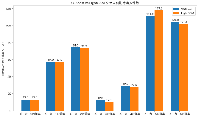
コード:クラス別に予測件数(期待件数)を出した結果可視化~可視化
# ------------------------------
# クラス別に予測件数(期待件数)を出した結果
# 確率列の抽出(0~6のクラス)
# ------------------------------
df_xgb_copy = df_merged.copy()
df_lgb_copy = df_lgb.copy()

prob_cols = [f"メーカー{i}の確率" for i in range(7)]

# ------------------------------
# 期待購入件数計算
# ------------------------------
xgb_expected = df_xgb_copy[prob_cols].sum().reset_index()
xgb_expected.columns = ["メーカー", "XGBoost 期待件数"]

lgb_expected = df_lgb_copy[prob_cols].sum().reset_index()
lgb_expected.columns = ["メーカー", "LightGBM 期待件数"]

# 結合
expected_df = pd.merge(xgb_expected, lgb_expected, on="メーカー")
print(expected_df)

# ------------------------------
# 可視化
# ------------------------------
x = np.arange(len(expected_df))
width = 0.35

fig, ax = plt.subplots(figsize=(10,6))
rects1 = ax.bar(x - width/2, expected_df["XGBoost 期待件数"], width, label="XGBoost")
rects2 = ax.bar(x + width/2, expected_df["LightGBM 期待件数"], width, label="LightGBM")

ax.set_ylabel("期待購入件数(確率ベース)")
ax.set_xticks(x)
ax.set_xticklabels(expected_df["メーカー"])
ax.set_title("XGBoost vs LightGBM クラス別期待購入件数")
ax.legend()

# 棒の上に数値表示
for rects in [rects1, rects2]:
    for rect in rects:
        height = rect.get_height()
        ax.annotate(f'{height:.1f}',
                    xy=(rect.get_x() + rect.get_width()/2, height),
                    xytext=(0,3),
                    textcoords="offset points",
                    ha='center', va='bottom')

plt.tight_layout()
plt.show()
出力例
       メーカー  XGBoost 期待件数  LightGBM 期待件数
0  メーカー0の確率     13.002707      12.995387
1  メーカー1の確率     56.987980      57.044848
2  メーカー2の確率     74.000336      73.240391
3  メーカー3の確率     12.014658      10.133637
4  メーカー4の確率     29.020639      27.607897
5  メーカー5の確率    110.991791     117.337932
6  メーカー6の確率    103.981888     101.639907
コード: LightGBM SHAP値~可視化
# 寄与度比較
# ========================
# LightGBM SHAP値
# ========================
lgb_explainer = shap.TreeExplainer(lgb_model)
shap_lgb_values = lgb_explainer.shap_values(X_df)

# binary/multiclass の処理
if isinstance(shap_lgb_values, list):
    shap_lgb_array = np.array([shap_lgb_values[pred][i,:] for i,pred in enumerate(df_lgb["predicted_class"])])
else:
    shap_lgb_array = shap_lgb_values

shap_lgb_df = pd.DataFrame(np.abs(shap_lgb_array).mean(axis=0), index=X_df.columns, columns=["LightGBM"])

# ========================
# XGBoost SHAP値
# ========================
X_df_enc = X_df.copy()
for col in X_df_enc.select_dtypes(include="category"):
    X_df_enc[col] = X_df_enc[col].cat.codes

xgb_explainer = shap.TreeExplainer(xgb_model)
shap_xgb_values = xgb_explainer.shap_values(X_df_enc)

if isinstance(shap_xgb_values, list):
    shap_xgb_array = np.array([shap_xgb_values[pred][i,:] for i,pred in enumerate(df_xgb["predicted_class"])])
else:
    shap_xgb_array = shap_xgb_values

shap_xgb_df = pd.DataFrame(np.abs(shap_xgb_array).mean(axis=0), index=X_df_enc.columns, columns=["XGBoost"])

# ========================
# 比較
# ========================
shap_compare = shap_xgb_df.join(shap_lgb_df).sort_values("XGBoost", ascending=False)
print(shap_compare)

# ========================
# 可視化(棒グラフ)
# ========================
# 横棒グラフで可視化
#shap_compare.plot(kind="barh", figsize=(10, 8), width=0.7)

shap_compare.plot(kind="bar", figsize=(12,6))
plt.ylabel("平均SHAP値(寄与度)")
plt.title("XGBoost vs LightGBM 寄与度比較")
plt.xticks(rotation=45, ha="right")
plt.tight_layout()
plt.show()
出力例
                        XGBoost  LightGBM
income                 1.260725  1.822286
car_preference         1.028896  1.118688
previous_manufacturer  0.728317  0.446252
age                    0.383150  0.309408
hobby                  0.321610  0.170742
region                 0.205471  0.242472
family                 0.147715  0.129417
gender                 0.105472  0.090702
children               0.055276  0.086637
employment_type        0.049248  0.062799
previous_car_owner     0.030030  0.114660
test_drive             0.028128  0.008967
marital_status         0.000000  0.028145

📌精度と特徴量寄与の比較
❓指標の意味❓
Top-k 精度
- Top-1 精度:1位の予測が正解と一致した割合(Accuracy に近い)
-
Top-3 精度:予測上位3位のいずれかが正解と一致した割合
- 「正解が候補上位に入っているか」を確認できる
Accuracy / F1 Score
- Accuracy = 正解と一致した割合
- F1 Score = クラス間の不均衡を考慮した平均精度
- Top-1 精度と概念的に近い
✅ 全体精度(今回のデータ)
- Top-1 精度は LightGBM 0.73、XGBoost 0.72(例)
- Top-3 精度もほぼ同等
- 精度だけを見ると、両モデルに大きな差はない
✅ クラス別精度
- XGBoost:全クラスで安定して高い精度
- LightGBM:一部のクラスで高い精度、低い精度のばらつきあり
✅ 特徴量寄与(SHAP値)
- XGBoost:主要特徴量に寄与が集中、少数の特徴量で判断
- LightGBM:カテゴリを含め、上位特徴量がいくつかに分散
✅ 結論
- 精度だけなら両モデルほぼ同じ
- SHAP値を見ると、モデルごとに特徴量の使い方に違いがある
- データや目的に応じて、精度・解釈性・速度のバランスで選ぶのが現実的
- 実務では両方試して比較するのが安心
📌まとめ
もう少し情報があれば、販売予測も可能です。
サンプルデータの準備できたら、予測パートも投稿する予定です。
Discussion