🍓

Strong bias arising from extremely difficult regression problems 考察

2022/12/20に公開

この記事は仮想通貨botter Advent Calendar 2022 22日目の記事です。

去年に引き続きアドベントカレンダーやっていきます。

まえがき

もともとは、時系列の効率的なメモリであるHiPPO/S4の理論解説と実装を紹介する予定でしたが、3日目の記事で紹介されていたノイズにより回帰がうまく機能しない問題が面白そうだったため、今回はラベルノイズが回帰に与える影響について考えたいと思います。面白い問題を提案してただきありがとうございます！

問題設定

問題設定はrichwomanbtcの記事がわかりやすいです。
端的に書くと、回帰問題で $x\in\mathbb{R}^{d}$ , $y\in\mathbb{R}$ としたときに

\begin{aligned} y'&=f\left(x\right)+\varepsilon\\ y&=\frac{y'}{Var\left[y'\right]}\\ \varepsilon&\sim N\left(0,\alpha\right) \end{aligned}

ここで $f$ は決定的な関数, $\varepsilon$ はガウスノイズ。 $E[y]=0$ でノイズの強さ $\alpha$ が大きいときに、回帰問題を解くと、予測の平均が0に集中してしまうという問題です。

コード

import random
import numpy as np
import torch
import torch.nn as nn
import torch.nn.functional as F
import pandas as pd
import skorch
from skorch.callbacks import Callback, Checkpoint, EarlyStopping
from skorch.dataset import CVSplit
from sklearn.model_selection import train_test_split
import holoviews as hv
from holoviews import opts
hv.extension('bokeh')

opts.defaults(opts.Histogram(alpha=0.5, width=600), opts.Overlay(width=600, legend_position='right'))


def torch_fix_seed(seed=42):
    # Python random
    random.seed(seed)
    # Numpy
    np.random.seed(seed)
    torch.manual_seed(seed)
    torch.cuda.manual_seed(seed)
    torch.backends.cudnn.deterministic = True
    torch.use_deterministic_algorithms = True
torch_fix_seed()

def get_y(d, df):
    net = nn.Sequential(
        nn.Linear(d, 100, bias=False),
        nn.Tanh(),
        nn.Linear(100, 1, bias=False)
    )

    train_data = torch.tensor(np.array(df.astype('f')))
    y = pd.Series(net(train_data).detach().numpy().reshape(-1))
    y /= dist_factor*y.std() # normalize
    return y

net = nn.Sequential(
    nn.Linear(d, 100, bias=False),
    nn.Tanh(),
    nn.Linear(100, 1, bias=False)
)


monitor = lambda Net: all(Net.history[-1, ('train_loss_best', 'valid_loss_best')])
 
# set param(make trainer)
model = skorch.regressor.NeuralNetRegressor(
                    net,
                    max_epochs=500,
                    lr=0.005,
                    warm_start=True,
                    optimizer=torch.optim.Adam,
                    #optimizer=torch.optim.SGD,
                    #optimizer__momentum=0.9,
                    iterator_train__shuffle=True,
                    callbacks=[Checkpoint(), EarlyStopping()],
                    train_split=CVSplit(cv=4)
                )

def create_model(d):
    net = nn.Sequential(
    nn.Linear(d, 100, bias=False),
    nn.Tanh(),
    nn.Linear(100, 1, bias=False)
    )
    model = skorch.regressor.NeuralNetRegressor(
                    net,
                    max_epochs=500,
                    lr=0.005,
                    warm_start=True,
                    optimizer=torch.optim.Adam,
                    #optimizer=torch.optim.SGD,
                    #optimizer__momentum=0.9,
                    iterator_train__shuffle=True,
                    callbacks=[Checkpoint(), EarlyStopping()],
                    train_split=CVSplit(cv=4)
                )
    return model
def get_results(d, N, alpha, dist_factor=1, train_size=0.5):
    ret = {}
    model = create_model(d)
    df = pd.DataFrame(np.random.normal(size=[N, d]).astype('float32'), columns=[f"feat_{i}" for i in range(d)])
    y = get_y(d, df)
    if alpha == 0:
        noisy_y = y.values
    else:
        noisy_y = y.values + np.random.normal(size=y.shape, scale=alpha).astype('float32')
    noisy_y = noisy_y / noisy_y.std()/dist_factor
    if train_size == 1.0:
        train_df = df
        test_df = df
        train_noisy_y = noisy_y
        test_noisy_y = noisy_y        
    else:
        train_df, test_df = train_test_split(df, train_size=train_size)
        train_noisy_y, test_noisy_y = train_test_split(noisy_y, train_size=train_size)    
    
    model.fit(train_df.values, train_noisy_y.reshape(-1, 1))
    pred = pd.Series(model.predict(test_df.values).flatten())
    print(f"---")
    print(f"noise level: {alpha}")
    print(f"MSE: {np.mean((pred - test_noisy_y)**2):.3f}")
    print(f"target mean: {test_noisy_y.mean():.3f}, std: {test_noisy_y.std():.3f}")
    print(f"pred mean: {pred.mean():.3f}, std: {pred.std():.3f}, std: {pred.std():.3f}")
    print(f"SNR: {((pred - test_noisy_y.mean())**2 ).sum()/ ((test_noisy_y - pred)**2).sum()}")
    print(f"---")
    ret['noisy_level'] = alpha
    ret['mse'] = np.mean((pred - test_noisy_y)**2)
    ret['target_mean'] = test_noisy_y.mean()
    ret['target_std'] = test_noisy_y.std()    
    ret['pred_mean'] = pred.mean()
    ret['pred_std'] = pred.std()    
    ret['snr'] = ((pred - test_noisy_y.mean())**2 ).sum()/ ((test_noisy_y - pred)**2).sum()
    ret['test_x'] = test_df
    ret['test_y'] = test_noisy_y    
    plot_dist(test_noisy_y, pred)
    return ret

$\alpha=0$ (これは異なるニューラルネットの初期値間を移動できるかの問題)だと

_ = get_results(d=100, N=5000, alpha=1, dist_factor=1, train_size=1)

なのに $\alpha=10$ だと

なぜこんなことが起きるのか？

以下の2つの問題がある

train(+validation)とtest dataがわけてないこと
ノイズを乗せたあとに分散を１に正規化していること

TrainとTestを分けた場合と分けなかった場合

元記事では学習で、trainとvalidationを分けていましたが、予測はholdout sampleになっていなかったです。これはoverfittingを引き起こします (ニューラルネットはlabelノイズが強い場合は特にoverfittingすることが知られています)。

trainとtestを分けた場合そもそももとの分布をちゃんとfitできない
元記事の設定に合わせた実験でノイズなしの場合

trainとtestをわけない

get_results(d=10, N=10000, alpha=0, dist_factor=1.0, train_size=1)

MSE: 0.001
target mean: -0.005, std: 1.000
pred mean: -0.005, std: 0.999, std: 0.999
SNR: 846.236328125

trainとtestを50%づつに分ける

get_results(d=10, N=10000, alpha=0, dist_factor=1.0, train_size=0.5)

MSE: 1.024
target mean: 0.007, std: 1.005
pred mean: -0.000, std: 0.125, std: 0.125
SNR: 0.015294821001589298

これは過学習しているため起きている。ノイズが乗っている場合は一見正しく予測できてそうに見えているがそうではない。

データ数やNNのパラメータを頑張ってチューンすると解決するかも？　future work
今回は回帰問題だが、分類問題でもノイズにより過学習することが研究で調べられている。
ノイズが多い場合からくる過学習対策の手法は回帰と分類それぞれの場合で多くの論文が提案されているためそういうのを試すといいかも

trainとtestを分けて場合のいろんなパラメータでの実験結果

train dataに対してplotした場合
train N: 5000
d: 100
alpha: 0

MSE: 0.082
target mean: -0.030, std: 2.000
pred mean: -0.029, std: 1.950, std: 1.950
SNR: 46.62129211425781

train N: 5000
d: 100
alpha: 10

MSE: 3.644
target mean: 0.020, std: 2.000
pred mean: -0.007, std: 0.583, std: 0.583
SNR: 0.09348120540380478

trainとtestに50%ずつでわけて、testに対してpredした場合
train N: 2500
test N: 2500
d: 100
alpha=0

MSE: 4.297
target mean: 0.027, std: 2.006
pred mean: 0.001, std: 0.538, std: 0.538
SNR: 0.06747309863567352

alpha=10

alpha: 10
MSE: 111.611
target mean: 0.054, std: 10.270
pred mean: 0.012, std: 2.741, std: 2.741
SNR: 0.06729775667190552

trainとtestを50%に分けたことでデータ数が半分になっているため、データ数を倍にして学習データが1とおなじになるようにした
train N: 5000
test N: 5000
d: 100
alpha: 0

MSE: 4.107
target mean: -0.059, std: 1.992
pred mean: -0.006, std: 0.360, std: 0.360
SNR: 0.03229061886668205

alpha: 10

MSE: 109.304
target mean: 0.008, std: 10.302
pred mean: 0.055, std: 1.856, std: 1.856
SNR: 0.03153183311223984

ノイズを乗せたあと分散1への正規化の影響

ノイズを乗せて分散が大きくなった分布を正規化すると、もとのノイズが乗る前のデータが0に近づく

コード

N=10000
d=100
alpha = 10
df = pd.DataFrame(np.random.normal(size=[N, d]).astype('float32'), columns=[f"feat_{i}" for i in range(d)])
y = get_y(d, df)
noisy_y = y.values + np.random.normal(size=y.shape, scale=alpha).astype('float32')
y = noisy_y
pred = y/noisy_y.std()
frequencies, edges = np.histogram(pred, 50)
pred_plot = hv.Histogram((edges, frequencies), label='true_y')
frequencies, edges = np.histogram(y, 50)
y_plot = hv.Histogram((edges, frequencies), label='y')
hv.ipython.display(y_plot*pred_plot)

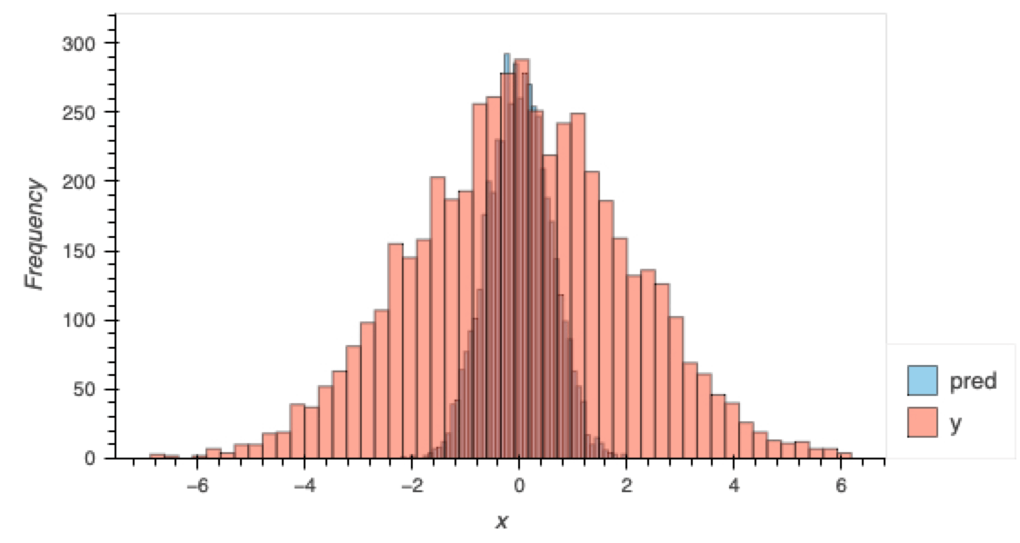
プロットすると

yと比較してノイズが乗っていないyが正規化の影響で0付近に寄っている。
よってそもそも0付近を予測することが正しい問題設定になっている。

ここで得た教訓は、ノイズが多いtargetを予測するときにデータごとにtargetの正規化を行ってしまうとノイズが乗る前のtargetは0付近に集中してしまうということである。(botでの利用の仕方次第では問題はないかもですが)

ノイズが多い場合の精度(MSE)の改善

botterは収益を出してなんぼなので、精度改善を行います。

以下trainとtestを分けて、ノイズにたいして正規化した場合

ノイズが多いデータを点推定しているのが問題だと思うので、確率密度推定を使います。
確率密度推定の手法であるVAEを教師あり学習に適当に改造してみる

普通ののVAEはこちらの記事が参考になります

真の分布を $p$ 、近似分布を $q$ とすると以下のように定式化できる

\begin{aligned} \log p\left(y|x\right)&=\int q\left(z|x\right)\log p\left(y|x\right)dz\\&=\int q\left(z|x\right)\log\frac{p\left(z,y,x\right)p\left(y,x\right)}{p\left(z,y,x\right)p\left(x\right)}dz\\&=\int q\left(z|x\right)\log\frac{p\left(z,y|x\right)}{p\left(z|x,y\right)}dz\\&=\int\left[q\left(z|x\right)\log\frac{q\left(z|x\right)}{p\left(z|x,y\right)}+q\left(z|x\right)\log\frac{p\left(z,y|x\right)}{q\left(z|x\right)}\right]dz\\&=D_{{\rm KL}}\left(q\left(z|x\right)||p\left(z|x,y\right)\right)+\int q\left(z|x\right)\log\frac{p\left(z,y|x\right)}{q\left(z|x\right)}dz\\&=D_{{\rm KL}}\left(q\left(z|x\right)||p\left(z|x,y\right)\right)+\int q\left(z|x\right)\log\frac{p\left(y,x|z\right)p\left(z\right)}{q\left(z|x\right)p\left(x\right)}dz\\&=D_{{\rm KL}}\left(q\left(z|x\right)||p\left(z|x,y\right)\right)-D_{{\rm KL}}\left(q\left(z|x\right)||p\left(z\right)\right)+\int q\left(z|x\right)\log p\left(y|x,z\right)dz\\&\geq\int q\left(z|x\right)\log p\left(y|x,z\right)dz-D_{{\rm KL}}\left(q\left(z|x\right)||p\left(z\right)\right) \end{aligned}

最後の出てきたのが変分下限で、これを最大化することで、下から2行目のzの事後分布が真の分布と一致します。
最後の行の第一項目は分布を予測する項で、第2項は過学習を抑制する正則化項です。
$p(z)$ は仮定すべき事前分布で、普通はどうしようもないので標準ガウス分布を仮定します。
手前味噌ですが、確率密度推定においては、以前我々が提案した理論的に最適な事前分布をデータから推測する論文があるため今回はこれを使います。

decoderの分布をガウス分布としたとき、testデータ各点に対してp(y|x)は平均と分散を予測します。
test dataに対して予測した平均と分散から作ったガウス分布からサンプリングした場合
確率密度推定

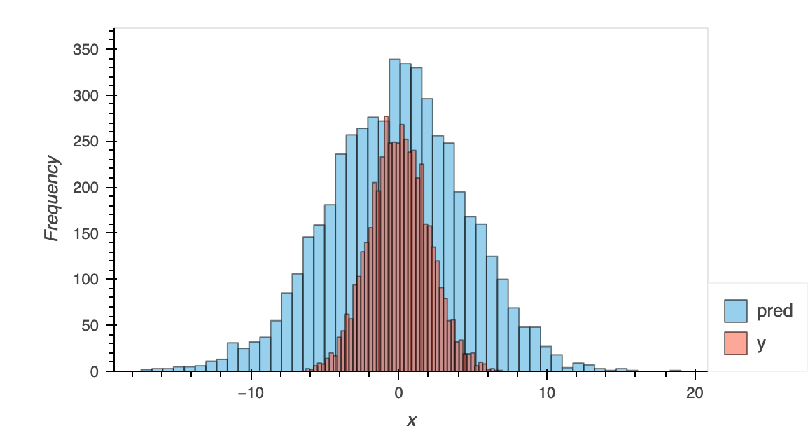
MSE 25.617846

平均値を使った場合

MSE 4.0318956

これは正解データが分散を正規化している問題から、ノイズが乗っていない $y$ は $0$ 近くにあり、それにノイズが乗っているため、各データ点ごとの平均は $0$ 近くを予測しています (よくみると0ではない値を出しています)

ここでデータ $y$ にのるノイズを考えるとデータ点ごとに大きいノイズが乗っているもの、小さいノイズが乗っているものが存在するはずです。つまり予測しやすい $\{x,y\}$ とそうでないものが混ざっているはずです。そこで予測された分散のなかから、分散が小さいものだけを使うという戦略が考えられます。
つまり自信がある点だけを使うという方法です。

$\log\alpha$

しきい値以下の分散に対応するデータ点を使ったときのMSE

しきい値	MSE
3.5	3.52
4.0	3.95
4.5	3.85
5.0	4.02
なし	4.03

データ点ごとの2乗のずれをみているため、結構改善されているのがわかります。
これはbotter的には、取引回数を下げて、自信があるものだけにベットして精度を上げることに対応します。
ポイントは、各点 $y$ を平均と分散を持った分布として予測しているところです。

[追加] regression vs classification

alphaを変えて0より大きいか0以下の2値のaccの変化をプロット
正規化は行っておらず、10 seedでエラーバーをつけた。
結果どっちを使ってもnoiseが大きくなると予測精度が下がり、有意差はなかった。

# Set the noise strengths
alphas_fine_low = np.linspace(0, 10, 10)

# Define dictionaries to store the accuracies for regression and classification
regression_accuracies_no_norm_low = {alpha: [] for alpha in alphas_fine_low}
classification_accuracies_no_norm_low = {alpha: [] for alpha in alphas_fine_low}

for iteration in range(n_iterations):
    for alpha in alphas_fine_low:
        # Generate the input from a standard normal distribution
        x = np.random.randn(n_samples, d)

        # Compute y' without normalization
        y_prime = f(x) + alpha * np.random.randn(n_samples, d)

        # Convert y' to binary labels
        y_labels = (y_prime >= 0).astype(int)

        # Split the data into a training set and a test set
        x_train, x_test, y_train, y_test = train_test_split(x, y_labels, test_size=0.2, random_state=42+iteration)

        # Train a logistic regression model
        model = LogisticRegression()
        model.fit(x_train, y_train.ravel())

        # Use the model to predict the output of the test data
        y_pred = model.predict(x_test)

        # Compute the accuracy of the predictions
        classification_accuracies_no_norm_low[alpha].append(accuracy_score(y_test, y_pred))

        # Now perform regression
        # Split the data into a training set and a test set
        x_train, x_test, y_train, y_test = train_test_split(x, y_prime, test_size=0.2, random_state=42+iteration)

        # Train a linear regression model
        model = LinearRegression()
        model.fit(x_train, y_train)

        # Use the model to predict the output of the test data
        y_pred = model.predict(x_test)

        # Convert the predictions and the true outputs to binary labels
        y_pred_labels = (y_pred >= 0).astype(int)
        y_test_labels = (y_test >= 0).astype(int)

        # Compute the accuracy of the predictions
        regression_accuracies_no_norm_low[alpha].append(accuracy_score(y_test_labels, y_pred_labels))

# Calculate means and standard deviations
regression_means_no_norm_low = {alpha: np.mean(accs) for alpha, accs in regression_accuracies_no_norm_low.items()}
classification_means_no_norm_low = {alpha: np.mean(accs) for alpha, accs in classification_accuracies_no_norm_low.items()}
regression_stds_no_norm_low = {alpha: np.std(accs) for alpha, accs in regression_accuracies_no_norm_low.items()}
classification_stds_no_norm_low = {alpha: np.std(accs) for alpha, accs in classification_accuracies_no_norm_low.items()}

# Plot the accuracies with error bars
plt.figure(figsize=(10, 6))
plt.errorbar(list(regression_means_no_norm_low.keys()), list(regression_means_no_norm_low.values()), yerr=list(regression_stds_no_norm_low.values()), label='Regression', capsize=5, color='red')
plt.errorbar(list(classification_means_no_norm_low.keys()), list(classification_means_no_norm_low.values()), yerr=list(classification_stds_no_norm_low.values()), label='Classification', capsize=5, color='blue')
plt.xlabel('Alpha (Noise Strength)')
plt.ylabel('Accuracy')
plt.legend()
plt.grid(True)
plt.title('Accuracy of Regression vs Classification with Different Noise Strengths (Alpha from 0 to 10)')
plt.show()