Binance永久先物の一時間足の基本的統計量と戯れる

きっかけ
[https://zenn.dev/wannabebotter/articles/a199233a6d6464](UKIさんのシストレのすすめを正座して読んで手を動かしてみる #3)では、対象とするマーケットの基本的統計量を見ることが大事だとわかりました。
せっかく約定履歴から一時間足を作れるようになったので、試しにBTCUSDTの基本的統計量が時間とともにどう変化しているかを見てみることにしました。
やること
- BTCUSDTの平均、標準偏差、歪度、尖度を7日間ローリングウィンドウで計算し、時間とともに基本的統計量がどのように変化しているかを確認する
- さらにそれらをADF検定し、定常性があるかを確認する
コードサンプル
このようなコードを利用して計算しました。
# ADF検定を実施する関数
def adf_stationary_test(target_series: pd.Series = None):
    _result = adfuller(target_series)
    _series_output = pd.Series(_result[0:4], index = ['Test Statistic', 'p-value', '#Lags Used', 'Number of Observations Used'])
    for _k, _v in _result[4].items():
        _series_output[f'Critical Value ({_k})'] = _v
    print(_series_output)
    print(f'This series is stationary : {_series_output["Test Statistic"] < _series_output["Critical Value (1%)"]}')
    return _series_output['Test Statistic'] < _series_output['Critical Value (1%)']
import pandas as pd
import statsmodels
from statsmodels.tsa.stattools import adfuller
import matplotlib.pyplot as plt
import japanize_matplotlib
import exercise_util

df_1h = exercise_util.concat_timebar_files('BTCUSDT', 3600)

df_1h['close'] = df_1h['close']

window_days = 7

df_1h['close_7days_mean'] = df_1h['close'].rolling(window_days * 24).mean()
df_1h['close_7days_std'] = df_1h['close'].rolling(window_days * 24).std()
df_1h['close_7days_skew'] = df_1h['close'].rolling(window_days * 24).skew()
df_1h['close_7days_kurt'] = df_1h['close'].rolling(window_days * 24).kurt()

df_1h.dropna(inplace = True)

plt.plot(df_1h.loc[df_1h.index > '2020-01-01', 'close_7days_mean'], label = 'df_1h.7days.mean', linewidth = 0.5)
plt.xticks(rotation = 45)
plt.legend()
plt.show()

exercise_util.adf_stationary_test(df_1h.loc[df_1h.index > '2020-01-01', 'close_7days_mean'])

plt.plot(df_1h.loc[df_1h.index > '2020-01-01', 'close_7days_std'], label = 'df_1h.7days.std', linewidth = 0.5)
plt.xticks(rotation = 45)
plt.legend()
plt.show()

exercise_util.adf_stationary_test(df_1h.loc[df_1h.index > '2020-01-01', 'close_7days_std'])

plt.plot(df_1h.loc[df_1h.index > '2020-01-01', 'close_7days_skew'], label = 'df_1h.7days.skew', linewidth = 0.5)
plt.xticks(rotation = 45)
plt.legend()
plt.show()

exercise_util.adf_stationary_test(df_1h.loc[df_1h.index > '2020-01-01', 'close_7days_skew'])

plt.plot(df_1h.loc[df_1h.index > '2020-01-01', 'close_7days_kurt'], label = 'df_1h.7days.kurt', linewidth = 0.5)
plt.xticks(rotation = 45)
plt.legend()
plt.show()

exercise_util.adf_stationary_test(df_1h.loc[df_1h.index > '2020-01-01', 'close_7days_kurt'])
コードサンプル全体はこちらです。
結果
平均

Test Statistic                    -1.723996
p-value                            0.418793
#Lags Used                        46.000000
Number of Observations Used    24768.000000
Critical Value (1%)               -3.430614
Critical Value (5%)               -2.861657
Critical Value (10%)              -2.566832
dtype: float64
This series is stationary : False
単なる7日間移動平均です。当然定常性はありません。
標準偏差

Test Statistic                -7.121902e+00
p-value                        3.703870e-10
#Lags Used                     4.800000e+01
Number of Observations Used    2.476600e+04
Critical Value (1%)           -3.430614e+00
Critical Value (5%)           -2.861657e+00
Critical Value (10%)          -2.566832e+00
dtype: float64
This series is stationary : True
かなり大きくなることはあるものの、比較的小さい値に戻ってくる性質が見てわかります。
定常性がある系列として判定されています。
時々大きな価格変化を起こしますが、連続して大きな価格変化が起こり続けることは少ない、ということでしょうか。
歪度

Test Statistic                -1.620665e+01
p-value                        4.025740e-29
#Lags Used                     1.900000e+01
Number of Observations Used    2.479500e+04
Critical Value (1%)           -3.430614e+00
Critical Value (5%)           -2.861657e+00
Critical Value (10%)          -2.566832e+00
dtype: float64
This series is stationary : True
見るからに定常性のある系列で、実際そのように判定されました。概ね平均0に戻ってくる性質があるようです。
時々ドッと上がったり下がったりする値動きが一方向によく見られるようになっても (歪度が正か負の大きな値に振れても) 、しばらくするとまたバランス良く上下動する動きに戻ってくる傾向があるようです (歪度が0近辺に戻ってくる)。
尖度

Test Statistic                   -20.127167
p-value                            0.000000
#Lags Used                         6.000000
Number of Observations Used    24808.000000
Critical Value (1%)               -3.430614
Critical Value (5%)               -2.861657
Critical Value (10%)              -2.566832
dtype: float64
This series is stationary : True
こちらも定常性ありと判定されています。まれに0以下の値になりますが、Ukiさんの記事にあるとおりほぼ正の値になっています。
時々鋭いスパイクのある値動きになりますが、そのような値動きはずっと続くことはない、ということでしょうか…。
おわりに
今回基本的統計量をローリングウィンドウでプロットしてみて、[https://zenn.dev/wannabebotter/articles/a199233a6d6464](UKIさんのシストレのすすめを正座して読んで手を動かしてみる #3) で銘柄ごとに一定の値を取るものとして計算した基本的統計量は、時間とともに大きく変化する値であることがわかりました。
また、標準偏差、歪度、尖度については、定常性があるケースもあるらしい、ということがわかりました。これらは値動きの様子を示す統計量なので、機械学習の特徴量として使いやすそうですし、工夫すればトレードロジックに組み込むこともできそうです。
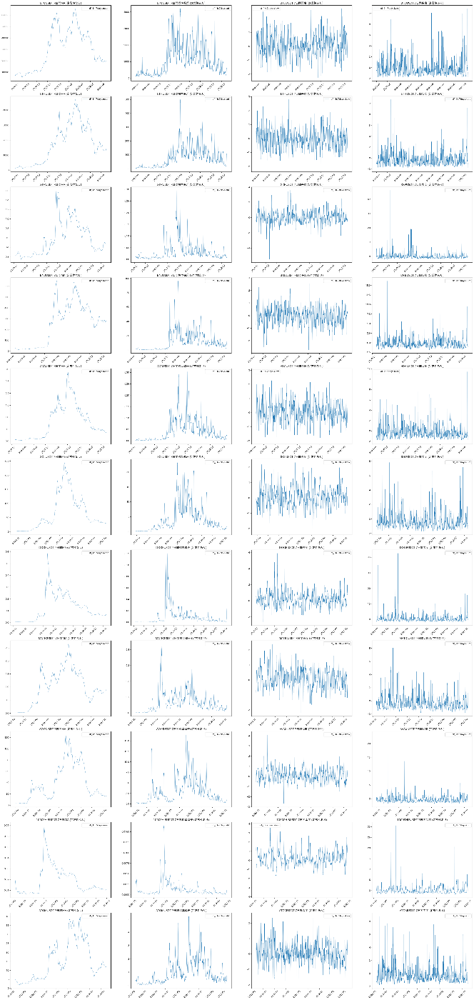
おまけ
複数銘柄について計算した結果の図はこちらです。どの銘柄も同じような傾向を示しています。
Discussion