【Python】resting stateの存在する化学反応の速度論シミュレーション

速度論シミュレーションのおさらい

化学反応の速度論シミュレーションでは、反応速度式（レート方程式）を連立して数値的に解く、という操作が一般に行われます。この際、4次のルンゲ＝クッタ法（RK4法）が用いられることが多く、先日これに関する記事を投稿しました。

https://zenn.dev/unyanyamine/articles/c4965b672a2ddb

本稿では、より複雑な反応素過程からなる系の速度論シミュレーションを実施します。

resting stateの存在する反応

"resting state"（休息状態）とは、副反応によって生じる比較的長寿命な中間体を指します。

例えば次のようなエネルギーダイアグラムで表現される反応系の場合、化学種Dがresting stateに相当します。

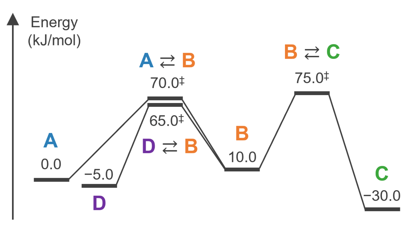
初期ポピュレーション（初期濃度）がAに100%存在する場合を考えます。反応が開始すると初めに中間体Bが生成し、その後速やかに中間体Dにポピュレーションが蓄積します。その後、生成物Cに全ポピュレーションが蓄積します。

$$\begin{array}{c} \large [\mathrm{A}] \, \underset{k_{1r}}{\overset{k_{1f}}{\rightleftarrows}} \, [\mathrm{B}] \, \underset{k_{2r}}{\overset{k_{2f}}{\rightleftarrows}} \, [\mathrm{C}] \\ \scriptsize{k_{3f}} \, \large{\downarrow \uparrow} \, \scriptsize{k_{3r}} \\ \large \overset{}{[\mathrm{D}]} \end{array}$$

この反応系のレート方程式は 300 K において次のようになります。

$$\begin{aligned} \dfrac{d[\mathrm{A}]}{dt} &= − 4.05 \times 10^{0} [\mathrm{A}] + 2.23 \times 10^{2} [\mathrm{B}] \\ \dfrac{d[\mathrm{B}]}{dt} &= 4.05 \times 10^{0} [\mathrm{A}] − 2.23 \times 10^2 [\mathrm{B}] − 3.01 \times 10^1 [\mathrm{B}] + 3.26 \times 10^{-6} [\mathrm{C}] - 1.65 \times 10^3 [\mathrm{B}] + 4.05 \times 10^0 [\mathrm{D}] \\ \dfrac{d[\mathrm{C}]}{dt} &= 3.01 \times 10^1 [\mathrm{B}] − 3.26 \times 10^{-6} [\mathrm{C}] \\ \dfrac{d[\mathrm{D}]}{dt} &= 1.65 \times 10^3 [\mathrm{B}] − 4.05 \times 10^0 [\mathrm{D}] \end{aligned}$$

【補足】
ここではすべての反応素過程を1次反応と仮定しています。

RK4法による速度論シミュレーション

以上の描像を実際に速度論シミュレーションによって確かめてみましょう。ここでは$10^{-4}$秒の刻み幅で$100$秒後までの濃度（ポピュレーション）の時間発展を調べてみます。

Pythonのコードは以下のようになります。

kinetic analysis by using RK4 method

import numpy as np
import matplotlib.pyplot as plt


k1f = 4.056047e+00
k1r = 2.234724e+02
k2f = 3.010672e+01
k2r = 3.267234e-06
k3f = 1.658762e+03
k3r = 4.056047e+00

def reaction_equations(concentrations):
    # Define the system of ordinary differential equations
    # Modify this function according to your specific reaction system
    A, B, C, D = concentrations
    dAdt = - k1f * A + k1r * B
    dBdt = k1f * A - k1r * B - k2f * B + k2r * C - k3f * B + k3r * D
    dCdt = k2f * B - k2r * C
    dDdt = k3f * B - k3r * D
    return [dAdt, dBdt, dCdt, dDdt]

def runge_kutta(dt, t_max, initial_concentrations):
    # Perform the simulation using the fourth-order Runge-Kutta method
    t = 0.0
    concentrations = np.array(initial_concentrations)
    time_points = [t]
    concentration_points = [concentrations]

    while t < t_max:
        # Compute concentration changes using the fourth-order Runge-Kutta method
        k1 = reaction_equations(concentrations)
        k2 = reaction_equations(concentrations + 0.5 * dt * np.array(k1))
        k3 = reaction_equations(concentrations + 0.5 * dt * np.array(k2))
        k4 = reaction_equations(concentrations + dt * np.array(k3))
        concentrations += (dt / 6.0) * (np.array(k1) + 2 * np.array(k2) + 2 * np.array(k3) + np.array(k4))
        t += dt

        time_points.append(t)
        concentration_points.append(concentrations.copy())

    return time_points, np.array(concentration_points)

# Example usage
dt = 1e-4  # Time step size
t_max = 1e+2  # Maximum simulation time
initial_concentrations = [1.0, 0.0, 0.0, 0.0]  # Initial concentrations of species A, B, C
time_points, concentration_points = runge_kutta(dt, t_max, initial_concentrations)
print(concentration_points[-1])

# Plotting the concentration curves
plt.plot(time_points[1:], concentration_points[1:, 0], label='A', color=(44/255, 127/255, 184/255))
plt.plot(time_points[1:], concentration_points[1:, 1], label='B', color=(237/255, 125/255, 49/255))
plt.plot(time_points[1:], concentration_points[1:, 2], label='C', color=(60/255, 167/255, 60/255))
plt.plot(time_points[1:], concentration_points[1:, 3], label='D', color=(112/255, 48/255, 160/255))
plt.xlabel('Time')
plt.ylabel('Concentration')
# plt.xscale('log')
# plt.yscale('log')
plt.legend()
plt.show()

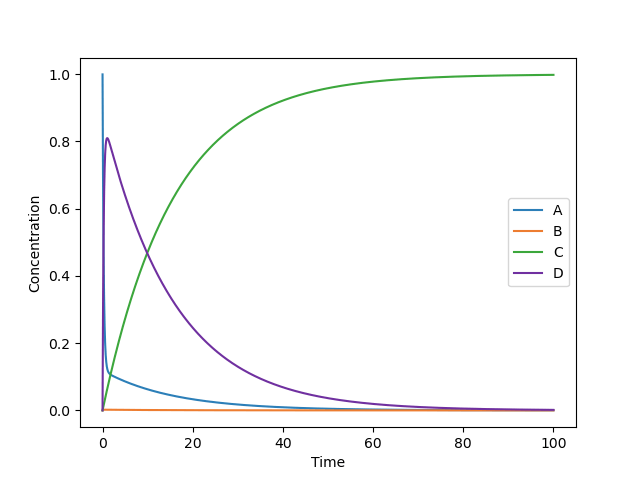
濃度の時間発展をプロットすると次のようになります。シミュレーションにより、100秒後の時点で約 99.8 %の反応物Aが生成物Cに変換されることが分かりました。

横軸を経過時間の対数として片対数グラフで描画すると次のようになります。

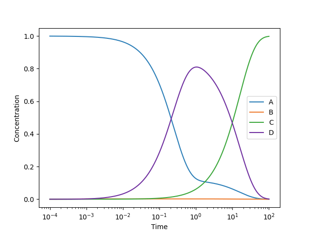
先ほどよりも短い時間スケールの濃度推移が見やすくなりましたね。1秒後の時点で約 81.0 %の反応物Aが中間体Dとして存在することが観察できます。つまり、うまく1秒で反応を停止できれば「速度論生成物」である中間体Dを高収量で得ることができそうです（自発的に反応が進行しない限りにおいて）。

ところで、この縦軸のスケールだと中間体Bが全く生成していないように見えます。しかしBは中間体として反応の過程で必ず経由しているので、ごく僅かながら濃度が存在するはずです。そこで縦軸も対数スケールにして両対数グラフとして描画してみましょう。

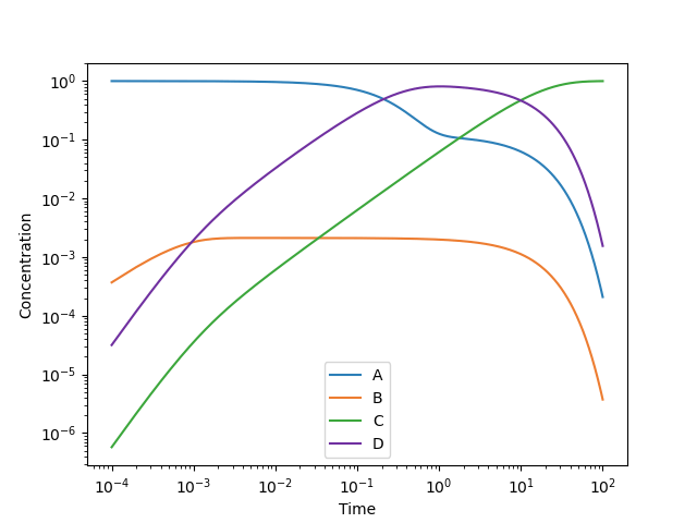
これを見ると、$10^{-3}$秒～$10$秒の範囲で約 0.2 %の濃度をもっていることが分かります。この時間帯において化学種Bについて定常状態が成立していることが視覚的に確認できます。

【補足】
一般に反応速度論によると、反応速度定数$k$は活性化エネルギー$\Delta G^{\ddagger}$の増大に対して指数的に減少することが知られています。この根拠となるのが以下の「アイリングの式」です。

$$k=\varGamma \, \dfrac{k_{\mathrm{B}}T}{h} \, \exp \left(-{\dfrac{\Delta G^{\ddagger}}{RT}}\right)$$

反応物が活性化障壁を超えるまでに要する時間は反応速度定数の逆数に比例するため、濃度（ポピュレーション）の時間発展を描画する際は横軸を反応時間の対数スケールとするのが合理的です。

---

※ 本稿はQiitaに投稿した記事「【Python】resting stateの存在する化学反応の速度論シミュレーション」に加筆して再投稿したものです。