Python+folium+openrouteserviceを使う (経路・時間行列・等時線を例に)
はじめに
以前,OSRM (Open Source Routing Machine) という道具を紹介しました.
自分で書いておいてなんですが,準備するのが面倒なのでWebサービス使いたいなという当たり前の気持ちになります.最近 openrouteservice という便利なサービスを使ってみたので,そちらを紹介します.
環境設定
openrouteserviceのページからアカウントを作成してAPIキーを取得します.Python用のライブラリとしてopenrouteserviceがあるのでインストールします.ついでにJupyter labで地図を可視化するためにfoliumをインストールしておきます.
pip install folium openrouteservice
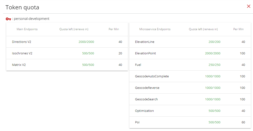
APIキーを取得すると,下の図のように各機能が利用できる回数が表示されています.
例えば経路検索に使うDirections V2 は,1日で無料の範囲で2000回 (1分で40回まで) 利用できることが分かります.
利用例
経路検索
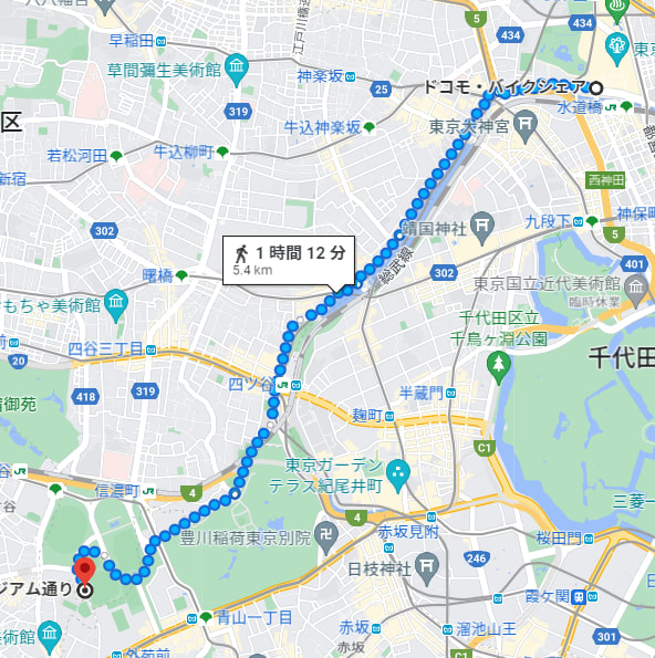
地点間の経路検索をやってみましょう.例として東京ドームの前から神宮球場まで移動する経路を探索してみます.Google Mapによれば
- 東京ドーム前
(35.70318768906786, 139.75197158765246) - 神宮球場前
(35.67431306373605, 139.71574523662844)
となります.openrouteservice を使うとき,緯度経度をひっくり返して渡す場面が多いので,注意が必要です.以下がプログラムです (APIキーは取得したやつを使います).
import folium
import openrouteservice
from branca.element import Figure
from openrouteservice import convert

key = "XXX"
client = openrouteservice.Client(key=key)

p1 = 35.70318768906786, 139.75197158765246
p2 = 35.67431306373605, 139.71574523662844
p1r = tuple(reversed(p1))
p2r = tuple(reversed(p2))
mean_lat = (p1[0] + p2[0]) / 2
mean_long = (p1[1] + p2[1]) / 2

# 経路計算 (Directions V2)
routedict = client.directions((p1r, p2r))
geom = routedict["routes"][0]["geometry"]
decoded = convert.decode_polyline(geom)
こうして計算した中身には経路の位置情報が含まれています.decodedの中身を確認してみると
{'type': 'LineString',
 'coordinates': [[139.75196, 35.70307],
  [139.75207, 35.70306],
  [139.75215, 35.70305],
  [139.75273, 35.703],
  [139.75322, 35.70296],
  [139.75338, 35.70295],
  ...
 ]}
このようになっています.これをfoliumのレイヤーとして追加すると経路を描画できます.
# 上の計算の続きで

def reverse_lat_long(list_of_lat_long):
    """緯度経度をひっくり返す"""
    return [(p[1], p[0]) for p in list_of_lat_long]

coord = reverse_lat_long(decoded["coordinates"])

# foliumでサイズ(600, 400)の地図を描画
fig = Figure(width=600, height=400)
m = folium.Map(location=(mean_lat, mean_long), zoom_start=13)
# 位置情報をPolyLineで地図に追加
folium.vector_layers.PolyLine(locations=coord).add_to(m)
fig.add_child(m)
次のような地図が作成できました.
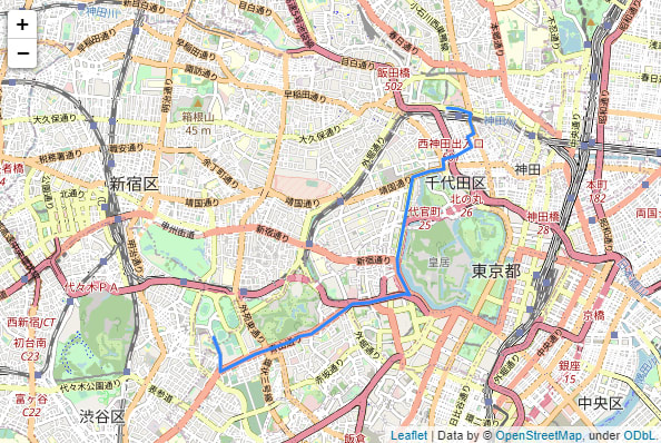
Google Mapとはだいぶ異なる結果が出ましたが,よく見るとGoogle Mapは徒歩ルートになっていました.そこでopenrouteserviceでも歩きルートを目指した検索をしてみます.directionsの関数にはprofileという引数があり,ここにprofile="foot-walking"と指定すると歩きの気持ちを考慮してくれます.foot-walkingで経路を引くと次のような経路が得られました.
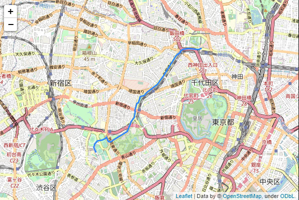
2つの結果を比較してみると…
| Googleマップ | Openrouteservice (foot-walking) |
|---|---|
|
|
最後のほうが少し違いますが,いい感じですね.ちなみにopenrouteserviceが返してくれる辞書には他の情報も含まれていて,routedict["routes"][0] を見てみると
{'summary': {'distance': 5493.6, 'duration': 3955.3},
 'segments': [{'distance': 5493.6,
   'duration': 3955.3,
   'steps': [{'distance': 17.2,
     'duration': 12.4,
     'type': 11,
     'instruction': 'Head west',
     'name': '-',
     'way_points': [0, 1]},
    {'distance': 37.1,
     'duration': 26.7,
     'type': 0, ######
}]]}
のように情報が得られます.この経路は5493.6[m]かつ3966.3[s]と言われています.距離はGoogleMapの5.4kmとほとんど同じです.GoogleMapの1時間12分は4320秒なので,時間に関しては5分ほどズレがありますね.
時間行列の取得
巡回セールスマン問題などを考えるとき,地点間の時間行列 (もしくは距離行列) があると便利なときがあります.
複数の地点 ({long, lat}) をopenrouteservice に投げると,行列で返してくれるAPIがdistance_matrix です.
以下に牛込柳町を中心に5地点を適当に選んだものを使って計算してみます.
# 牛込柳町あたりの5地点 (GoogleMapからコピペ)
p1 = 35.69978477165776, 139.72609683832815
p2 = 35.708984888401204, 139.7045104205496
p3 = 35.69992417527515, 139.73326370061565
p4 = 35.69264000939348, 139.72232028824695
p5 = 35.70609254178544, 139.72034618226493

lop = [p1, p2, p3, p4, p5]
ll = reverse_lat_long(lop)

# 徒歩による行列取得
dm_walking = client.distance_matrix(locations=ll, profile="foot-walking")
出力は次のようになります.
[[0.0, 2086.68, 658.19, 678.92, 845.32],
 [2086.68, 0.0, 2577.87, 2282.16, 1363.3],
 [658.19, 2577.87, 0.0, 1241.49, 1233.75],
 [678.92, 2282.16, 1241.49, 0.0, 1523.86],
 [845.32, 1363.3, 1233.75, 1523.86, 0.0]]
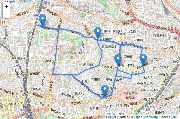
ちなみにこの5点の間でルートを引くと次のようになります.コードです.
routes = {}
for i in range(len(ll)):
    pi = ll[i]
    for j in range(i + 1, len(ll)):
        pj = ll[j]
        route_ij = client.directions((pi, pj))
        geom = route_ij["routes"][0]["geometry"]
        decoded = convert.decode_polyline(geom)
        routes[(i, j)] = reverse_lat_long(decoded["coordinates"])

# foliumで(600, 400)で可視化
fig = Figure(width=600, height=400)
m = folium.Map(location=(lat, long), zoom_start=14)

for i in range(len(ll)):
    pi = ll[i]
    folium.Marker(location=(pi[1], pi[0])).add_to(m)

for i in range(len(ll)):
    for j in range(i + 1, len(ll)):
        loc_ij = routes[(i, j)]
        folium.vector_layers.PolyLine(locations=loc_ij).add_to(m)
fig.add_child(m)
可視化結果です.
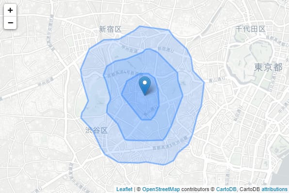
等時線マップ
日本語で何て言うのか正しく知らないのですが,Isochrones と呼ばれているものを計算します.ドキュメントによれば「Obtain areas of reachability from given locations」ですが,適当にGoogle検索すると等時線マップという日本語が引っかかりました.
先程の例で使った神宮球場を中心として,等時線マップを描画してみましょう.コードです.デフォルトの単位は時間 (秒) らしいので,神宮球場を中心に徒歩10分・20分・30分圏を描画しました.
fig = Figure(width=600, height=400)
p2 = 35.67431306373605, 139.71574523662844
m = folium.Map(location=(p2[0], p2[1]), tiles='cartodbpositron', zoom_start=13)

# 神宮球場 (long, latの順)
coordinate = [[p2[1], p2[0]]]

# isochrone
iso = client.isochrones(
    locations=coordinate,
    profile='foot-walking',
    range=[600, 1200, 1800],
    validate=False,
    attributes=["total_pop"]
)

folium.Marker(location=p2).add_to(m)

for isochrone in iso['features']:
    locs = [list(reversed(c)) for c in isochrone['geometry']['coordinates'][0]]
    folium.Polygon(locations=locs, fill='00ff00', opacity=0.5).add_to(m)
fig.add_child(m)
結果です.
まとめ
たまに使える気がします.
参考
公式サイトです.
例題や使い方を見たい場合にはpythonライブラリの使用例を見てください.
Discussion