【画像解析】Cellposeで顕微鏡写真から細胞をセグメンテーション2 - バッチ処理 -
前回、Cellpose GUIの使用方法やカスタムモデルの作成方法を紹介した。
しかし、Cellpose GUIではバッチ処理ができないため、せっかく汎用性のあるモデルができても他の画像に処理を繰り返すことができない。
本記事では、Pythonのコマンド処理でCellposeモデルを複数画像に適応する例を紹介する。
処理には前回作成したcellpose仮想環境を使用する。Anaconda Promptから仮想環境を立ち上げておく。
conda activate cellpose
このままコマンドラインで処理する方法と、Jupyter notebook/labを立ち上げて実行する方法がある。
【 コマンドラインから実行 】
python -m cellposeコマンドを使用する。
引数が沢山あるが、最低限使うものを以下に挙げる
-
--dir:
画像が入ったフォルダのパスを指定する。 -
--pretrained_model:
予測に使用するモデルの指定。cellposeで用意されているものであればモデル名、自身で作成した者であればモデルファイルへのパスを指定する。 -
--diameter:
検出したい構造/物体のピクセル直径。何も指定しなければ30が使用される。--diameter 0と指定すればモデルに保存された値を使用する。cellposeで用意されているモデルであれば画像ごとに予測してくれる?? -
--chan/--chan2:
使用するチャンネル番号。デフォルトは0でgrayscaleが想定されている。モデルによっては細胞質のチャンネル、核のチャンネルを指定することになる。 -
--savedir:
予測ラベル画像の保存先。指定しなければ--dirで指定したフォルダに予測結果が出力される。※ ただし予測ラベルのNumpyデータ「_seg.npy」ファイルは--dirのフォルダに保存される。 -
--save_png/--save_tif:
「_seg.npy」ファイルに加えて予測ラベルの画像をpngで保存するか、tifで保存するかを指示する。保存先は--savedirで指定した先。指定がなければ--dirのパスに保存される。 -
--save_rois:
ROIの輪郭座標情報のzipファイル。Cellpose GUIのFile > Save outlines as .zip archive of ROI files for ImageJで得られるものと同様で、ImageJのROI Managerから扱うことができる。 -
--use_gpu:
GPUを使うことを指示。GPU版Cellpose環境が用意できているならつけておく。
help
usage: __main__.py [-h] [--version] [--verbose] [--use_gpu] [--gpu_device GPU_DEVICE] [--check_mkl] [--dir DIR]
                   [--image_path IMAGE_PATH] [--look_one_level_down] [--img_filter IMG_FILTER]
                   [--channel_axis CHANNEL_AXIS] [--z_axis Z_AXIS] [--chan CHAN] [--chan2 CHAN2] [--invert]
                   [--all_channels] [--pretrained_model PRETRAINED_MODEL] [--add_model ADD_MODEL] [--unet]
                   [--nclasses NCLASSES] [--no_resample] [--net_avg] [--no_interp] [--no_norm] [--do_3D]
                   [--diameter DIAMETER] [--stitch_threshold STITCH_THRESHOLD] [--min_size MIN_SIZE] [--fast_mode]
                   [--flow_threshold FLOW_THRESHOLD] [--cellprob_threshold CELLPROB_THRESHOLD]
                   [--anisotropy ANISOTROPY] [--exclude_on_edges] [--augment] [--save_png] [--save_tif] [--no_npy]
                   [--savedir SAVEDIR] [--dir_above] [--in_folders] [--save_flows] [--save_outlines] [--save_rois]
                   [--save_ncolor] [--save_txt] [--train] [--train_size] [--test_dir TEST_DIR]
                   [--mask_filter MASK_FILTER] [--diam_mean DIAM_MEAN] [--learning_rate LEARNING_RATE]
                   [--weight_decay WEIGHT_DECAY] [--n_epochs N_EPOCHS] [--batch_size BATCH_SIZE]
                   [--min_train_masks MIN_TRAIN_MASKS] [--residual_on RESIDUAL_ON] [--style_on STYLE_ON]
                   [--concatenation CONCATENATION] [--save_every SAVE_EVERY] [--save_each]
                   [--model_name_out MODEL_NAME_OUT]

Cellpose Command Line Parameters

optional arguments:
  -h, --help            show this help message and exit
  --version             show cellpose version info
  --verbose             show information about running and settings and save to log

Hardware Arguments:
  --use_gpu             use gpu if torch with cuda installed
  --gpu_device GPU_DEVICE
                        which gpu device to use, use an integer for torch, or mps for M1
  --check_mkl           check if mkl working

Input Image Arguments:
  --dir DIR             folder containing data to run or train on.
  --image_path IMAGE_PATH
                        if given and --dir not given, run on single image instead of folder (cannot train with this
                        option)
  --look_one_level_down
                        run processing on all subdirectories of current folder
  --img_filter IMG_FILTER
                        end string for images to run on
  --channel_axis CHANNEL_AXIS
                        axis of image which corresponds to image channels
  --z_axis Z_AXIS       axis of image which corresponds to Z dimension
  --chan CHAN           channel to segment; 0: GRAY, 1: RED, 2: GREEN, 3: BLUE. Default: 0
  --chan2 CHAN2         nuclear channel (if cyto, optional); 0: NONE, 1: RED, 2: GREEN, 3: BLUE. Default: 0
  --invert              invert grayscale channel
  --all_channels        use all channels in image if using own model and images with special channels

Model Arguments:
  --pretrained_model PRETRAINED_MODEL
                        model to use for running or starting training
  --add_model ADD_MODEL
                        model path to copy model to hidden .cellpose folder for using in GUI/CLI
  --unet                run standard unet instead of cellpose flow output
  --nclasses NCLASSES   if running unet, choose 2 or 3; cellpose always uses 3

Algorithm Arguments:
  --no_resample         disable dynamics on full image (makes algorithm faster for images with large diameters)
  --net_avg             run 4 networks instead of 1 and average results
  --no_interp           do not interpolate when running dynamics (was default)
  --no_norm             do not normalize images (normalize=False)
  --do_3D               process images as 3D stacks of images (nplanes x nchan x Ly x Lx
  --diameter DIAMETER   cell diameter, if 0 will use the diameter of the training labels used in the model, or with
                        built-in model will estimate diameter for each image
  --stitch_threshold STITCH_THRESHOLD
                        compute masks in 2D then stitch together masks with IoU>0.9 across planes
  --min_size MIN_SIZE   minimum number of pixels per mask, can turn off with -1
  --fast_mode           now equivalent to --no_resample; make code run faster by turning off resampling
  --flow_threshold FLOW_THRESHOLD
                        flow error threshold, 0 turns off this optional QC step. Default: 0.4
  --cellprob_threshold CELLPROB_THRESHOLD
                        cellprob threshold, default is 0, decrease to find more and larger masks
  --anisotropy ANISOTROPY
                        anisotropy of volume in 3D
  --exclude_on_edges    discard masks which touch edges of image
  --augment             tiles image with overlapping tiles and flips overlapped regions to augment

Output Arguments:
  --save_png            save masks as png and outlines as text file for ImageJ
  --save_tif            save masks as tif and outlines as text file for ImageJ
  --no_npy              suppress saving of npy
  --savedir SAVEDIR     folder to which segmentation results will be saved (defaults to input image directory)
  --dir_above           save output folders adjacent to image folder instead of inside it (off by default)
  --in_folders          flag to save output in folders (off by default)
  --save_flows          whether or not to save RGB images of flows when masks are saved (disabled by default)
  --save_outlines       whether or not to save RGB outline images when masks are saved (disabled by default)
  --save_rois           whether or not to save ImageJ compatible ROI archive (disabled by default)
  --save_ncolor         whether or not to save minimal "n-color" masks (disabled by default
  --save_txt            flag to enable txt outlines for ImageJ (disabled by default)

Training Arguments:
  --train               train network using images in dir
  --train_size          train size network at end of training
  --test_dir TEST_DIR   folder containing test data (optional)
  --mask_filter MASK_FILTER
                        end string for masks to run on. use "_seg.npy" for manual annotations from the GUI. Default:
                        _masks
  --diam_mean DIAM_MEAN
                        mean diameter to resize cells to during training -- if starting from pretrained models it
                        cannot be changed from 30.0
  --learning_rate LEARNING_RATE
                        learning rate. Default: 0.2
  --weight_decay WEIGHT_DECAY
                        weight decay. Default: 1e-05
  --n_epochs N_EPOCHS   number of epochs. Default: 500
  --batch_size BATCH_SIZE
                        batch size. Default: 8
  --min_train_masks MIN_TRAIN_MASKS
                        minimum number of masks a training image must have to be used. Default: 5
  --residual_on RESIDUAL_ON
                        use residual connections
  --style_on STYLE_ON   use style vector
  --concatenation CONCATENATION
                        concatenate downsampled layers with upsampled layers (off by default which means they are
                        added)
  --save_every SAVE_EVERY
                        number of epochs to skip between saves. Default: 100
  --save_each           save the model under a different filename per --save_every epoch for later comparsion
  --model_name_out MODEL_NAME_OUT
                        Name of model to save as, defaults to name describing model architecture. Model is saved in
                        the folder specified by --dir in models subfolder.
1. モデルの用意
前回に引き続き、位相差顕微鏡の明視野画像を使用し、モデルもカスタムで作成したものを使用する。この記事では、デスクトップに「models/モデルファイル名」というような形で置いている想定である。
pretrainedモデルを使う場合は、モデル名を指定するとモデルファイルをダウンロードしてくれる。
2. 予測用画像フォルダの用意
まず予測したい画像を入れたフォルダを用意する。分かりやすいようにデスクトップにフォルダを配置している。

3. 予測の実行
次のコマンドを実行。--dir引数に予測用画像フォルダのパス、--pretrained_model引数にモデルファイルのパスを指定する。(絶対パスが望ましいみたい)
python -m cellpose --dir "C:\Users\Ryota_Chijimatsu\Desktop\Prediction" --pretrained_model C:\Users\Ryota_Chijimatsu\Desktop\models\CP_20230728_122230 --chan 0 --chan2 0 --diameter 0 --save_png --save_rois

実行画面
4. 結果の確認
終了すると、以下のような出力が得られる。
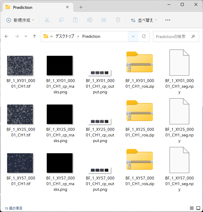
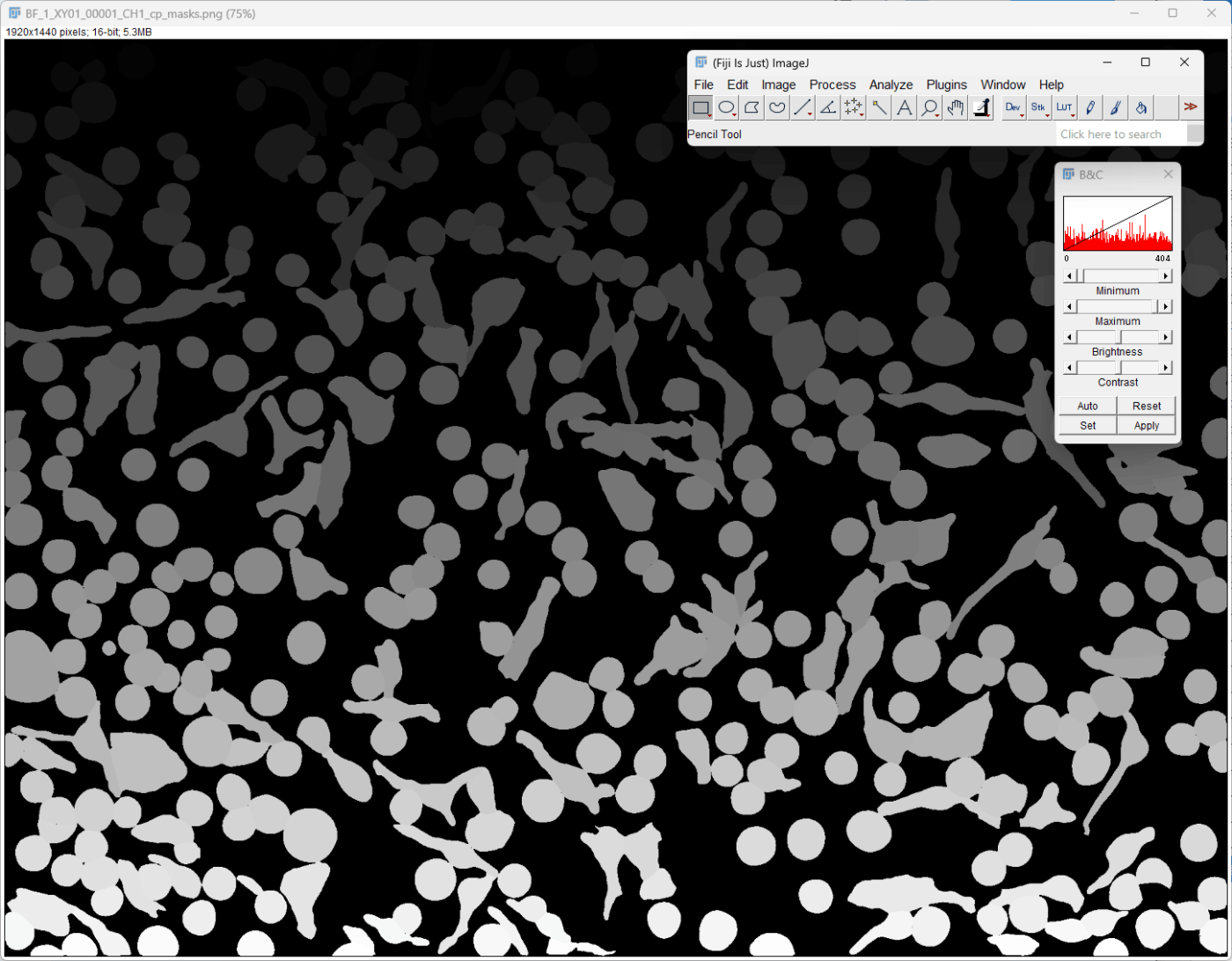
「_cp_masks.png」で終わるファイルはImageJで開いてみると検出された細胞ごとに異なる輝度を持つラベル画像であることが確認できる。
「_cp_output.png」で終わるファイルは予測のサマリー画像を並べて表示している。

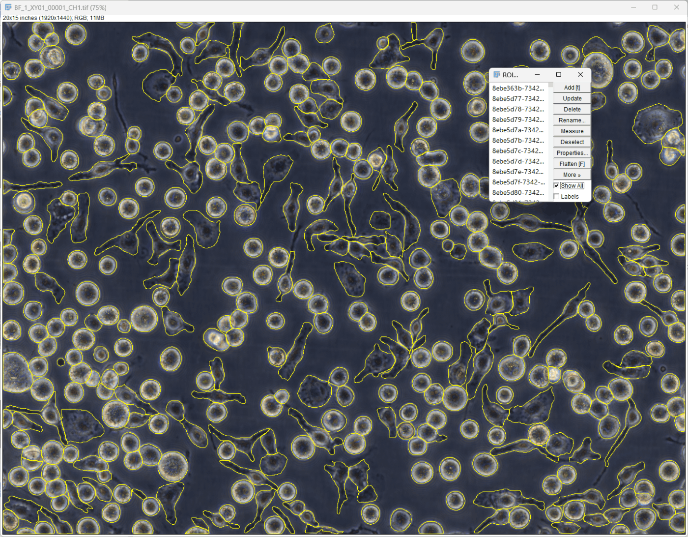
「_rois.zip」ファイルはImageJで扱うROI情報である。(ImageJで元画像を開く -> Analyze > Tools > ROI Manager -> ROI ManagerのMore > OpenからRoiのzipファイルを開く。)
【 Notebookから実行 】
https://cellpose.readthedocs.io/en/latest/notebook.html
https://nbviewer.org/github/MouseLand/cellpose/blob/master/notebooks/run_cellpose.ipynb
こちらの本でも紹介していますのでご参照ください。
まずはJupyter notebookかJupyter labを立ち上げる。
jupyter lab
1. ライブラリ読み込み
cellposeの中のmodelsモジュールで予測モデルの読み込み、予測の実行を行う。
ioモジュールは予測用画像の読み込み、予測結果の書き出しに使用する。
from cellpose import models, io
2. モデルの読み込み
.CellposeModel()メソッドを使用して、モデルを読み込む。cellposeで用意されたモデルを使用する際はmodel_type='cyto'のように指定する。
カスタムモデルを使用する際はpretrained_model=引数でモデルファイルのパスを指定する。
model_path = r"C:\Users\Ryota_Chijimatsu\Desktop\models\CP_20230728_122230"
model = models.CellposeModel(pretrained_model=model_path)
3. 予測画像の読み込み
予測に使用する画像を読み込む。cellposeのio.imreadを使うが、numpy配列の画像データが得られれば他のツールでもよい。
予測には1枚の画像か、複数の画像のリストを使用する。
img_path = r"C:\Users\Ryota_Chijimatsu\Desktop\Prediction\BF_1_XY01_00001_CH1.tif"
img = io.imread(filename=img_path)
from glob import glob

# 画像のファイルパスリスト作成
img_list = glob(r"C:\Users\Ryota_Chijimatsu\Desktop\Prediction\*.tif")

# 画像リストに変換
img_list = [ io.imread(img) for img in img_list]
4. 予測の実行
.eval()メソッドを使用する。引数には 1枚の画像か画像リスト、diameter=やchannels=引数などを使用する。
diameter=Noneとすると物体の直径を自動で見繕ってくれる。
channels=引数では[channel1の番号, channel2の番号]のようなリストで指定する。番号0はgrayscaleかNoneを意味する。モデルによって変わるのでモデルが訓練したチャンネルの情報を知っておく必要がある。

予測の実行とその出力を確認してみる。
result1 = model.eval(x=img,
                    diameter=None,
                    channels=[0,0])
result2 = model.eval(x=img_list,
                    diameter=None,
                    channels=[0,0])
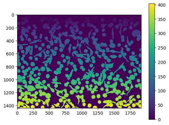
5. 結果の確認
結果は複数の返り値を受け取っている。
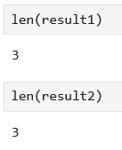
そのうちの1つ目の返り値が予測されたラベル画像となる。
plt.imshow(result1[0])
plt.colorbar()
画像リストで予測した場合は、1つ目の返り値もラベル画像のリストとなっている。
fig, axs = plt.subplots(1,3, figsize=(10,10))
axs[0].imshow(result2[0][0])
axs[1].imshow(result2[0][1])
axs[2].imshow(result2[0][2])

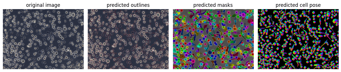
予測結果のサマリー
必要であれば、次のように予測結果の情報を使って、サマリー画像を確認できる。
from cellpose import plot
import matplotlib.pyplot as plt # pip install matplotlib

fig = plt.figure(figsize=(12,5))
plot.show_segmentation(fig, img=img, maski=result1[0], flowi=result1[1][0])
plt.tight_layout()
plt.show()
6. 結果の書き出し
io.masks_flows_to_seg()機能を使って、「_seg.npy」ファイルをローカルに書き出す。
io.masks_flows_to_seg(images=img, masks=result1[0], flows=result1[1], diams=None, file_names="tmp")
io.save_to_png()機能で予測ラベル画像を書き出す。
io.save_to_png(images=img, masks=result1[0], flows=result1[1], file_names="label.png")
【 QuPathでCellpose 】
QuPathという無料の画像解析ソフトにCellpose拡張機能が公開されている。
詳細は私の本で紹介している。
cellposeの公開済みモデルを使って複数の画像/領域に予測を行うことができるだけでなく、Cellpose GUIで作成したモデルをQuPathで使うこともできる。
さらにはQuPath内で予測モデルを作ることも可能。Cellpose GUIよりもアノテーションツールが豊富であり、ラベル付けも行いやすい。
Whole slide imageのような大きなデータでも、画像中の任意の箇所にラベル付けをしてモデルの学習が行える。
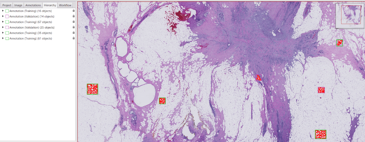
正解ラベルの例
明視野画像でCellposeを使うとグレースケール画像が使われるが、QuPathでカラーデコンボリューションしてヘマトキシリンチャンネルやDABチャンネルをCellposeに使うこともできる。
Discussion