🌊
東工大機械系院試をpythonで解いてみた[流体力学編]


はじめに
東工大の機械系の院試の問題をpythonを使って解いてみます。今回は令和1年度 流体力学 問題1を解いていきます。過去問は以下のページにあります。
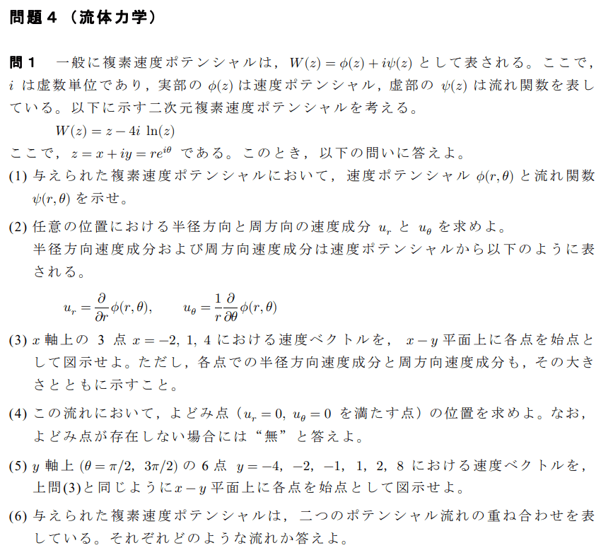
問題
(1)
from sympy import symbols, I, ln, cos, sin, re, im, arg, Abs

# 変数 r と theta を定義
r, theta = symbols('r theta')

# z = r(cos(theta) + i*sin(theta)) を定義
z = r * (cos(theta) + I*sin(theta))

# W(z) = z - 4i*ln(z) を定義し、z を代入
W_z = z - 4*I*ln(z)
W_z_substituted = W_z.subs(z, r*(cos(theta) + I*sin(theta)))

# 式を展開
W_z_expanded = W_z_substituted.expand()

# 実部と虚部を取得
phi = W_z_expanded.as_real_imag()[0]
psi = W_z_expanded.as_real_imag()[1]

# 実部の式を簡略化
phi_simplified = phi.subs([(re(r*cos(theta)), r*cos(theta)),
                           (im(r*sin(theta)), 0),
                           (arg(r*(I*sin(theta) + cos(theta))), theta)])

# 虚部の式を簡略化
psi_simplified = psi.subs([(Abs(I*r*sin(theta) + r*cos(theta)), r),
                           (re(r*sin(theta)), r*sin(theta)),
                           (im(r*cos(theta)), 0)])

# 簡略化された実部と虚部の式を表示
phi_simplified, psi_simplified
答えは
となります。
(2)
問題文の導出より
from sympy import diff

u_r = diff(phi_simplified, r)
u_theta = 1/r *diff(phi_simplified, theta)

u_r, u_theta
答えは
となります。
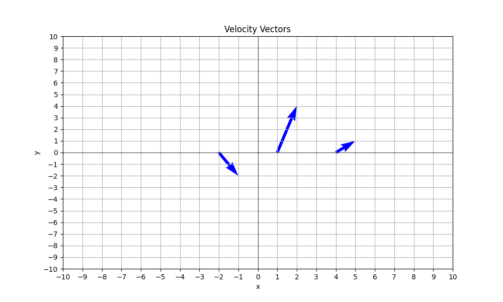
(3)
(2)の答えより、3点の速度ベクトルを求めます。
まず、各点での
from sympy import solve, pi, sqrt, atan2

r, theta, u_r, u_theta, u_x, u_y = symbols('r theta u_r u_theta u_x u_y')

# 与えられた値
u_r = cos(theta)
u_theta = 1/r * (4 - r*sin(theta))

# u_r と u_theta を u_x と u_y に変換
u_x = u_r*cos(theta) - u_theta*sin(theta)
u_y = u_r*sin(theta) + u_theta*cos(theta)

# x軸上の3点
x_values = [-2, 1, 4]
y_values = [0, 0, 0]

def compute_u_r_theta(x_value, y_value):
    #直交座標を極座標に変換する
    r_value = sqrt(x_value**2 + y_value**2)
    theta_value = atan2(y_value, x_value)
    # u_r, u_theta を計算
    u_r_value = u_r.subs([(r, r_value), (theta, theta_value)])
    u_theta_value = u_theta.subs([(r, r_value), (theta, theta_value)])
    size=sqrt(u_r_value**2 + u_theta_value**2)
    return u_r_value, u_theta_value, size

for x_value, y_value in zip(x_values, y_values):
     u_r_theta =compute_u_r_theta(x_value,y_value)
     print('(x,y)=({0},{1})でu_r={2},u_theta={3} 大きさ {4}'.format(x_value, y_value,u_r_theta[0],u_r_theta[1],u_r_theta[2]))

#出力結果
# (x,y)=(-2,0)でu_r=-1,u_theta=2 大きさ sqrt(5)
# (x,y)=(1,0)でu_r=1,u_theta=4 大きさ sqrt(17)
# (x,y)=(4,0)でu_r=1,u_theta=1 大きさ sqrt(2)
図示します。
import matplotlib.pyplot as plt
import numpy as np

u_x_values = []
u_y_values = []

#図示するため、x,y方向の速度ベクトルを求める
def velocity_vector_cartesian(x, y):
    r = sqrt(x ** 2 + y ** 2)
    theta = atan2(y, x)
    u_r = cos(theta)
    u_theta = 1/r * (4 - r*sin(theta))
    u_x_value = u_r * cos(theta) - u_theta * sin(theta)
    u_y_value = u_r * sin(theta) + u_theta * cos(theta)

    u_x_value =float(u_x_value)
    u_y_value =float(u_y_value)

    u_x_values.append(u_x_value)
    u_y_values.append(u_y_value)

for x_value, y_value in zip(x_values, y_values):
    velocity_vector_cartesian(x_value,y_value)

# グリッド間隔1でプロットを作成する
plt.figure(figsize=(10, 6))
plt.quiver(x_values, y_values, u_x_values, u_y_values, angles='xy', scale_units='xy', scale=1, color='b')
plt.xlim(-10, 10)
plt.ylim(-10, 10)
plt.axhline(0, color='black', linewidth=0.5)
plt.axvline(0, color='black', linewidth=0.5)
plt.grid(True)
plt.xticks(np.arange(-10, 11, 1))
plt.yticks(np.arange(-10, 11, 1))
plt.xlabel('x')
plt.ylabel('y')
plt.title('Velocity Vectors')
plt.show()
(4)
# u_r = 0となるθを求める
theta_stagnation = solve(u_r, theta)
# 0 <= θ <= 2πの範囲内にある値だけを保持する
theta_stagnation = [t for t in theta_stagnation if 0 <= t <= 2*pi]

# 求めたθとu_theta = 0からrを求める
r_stagnation = [solve(u_theta.subs(theta, t), r) for t in theta_stagnation]

print(r_stagnation)#[[4], [-4]] rは正の値を取るのでr=4
# 極座標を直交座標に変換する
x_stagnation = r_stagnation[0][0] * cos(theta_stagnation[0])
y_stagnation = r_stagnation[0][0] * sin(theta_stagnation[0])

x_stagnation, y_stagnation
答えは
となります。
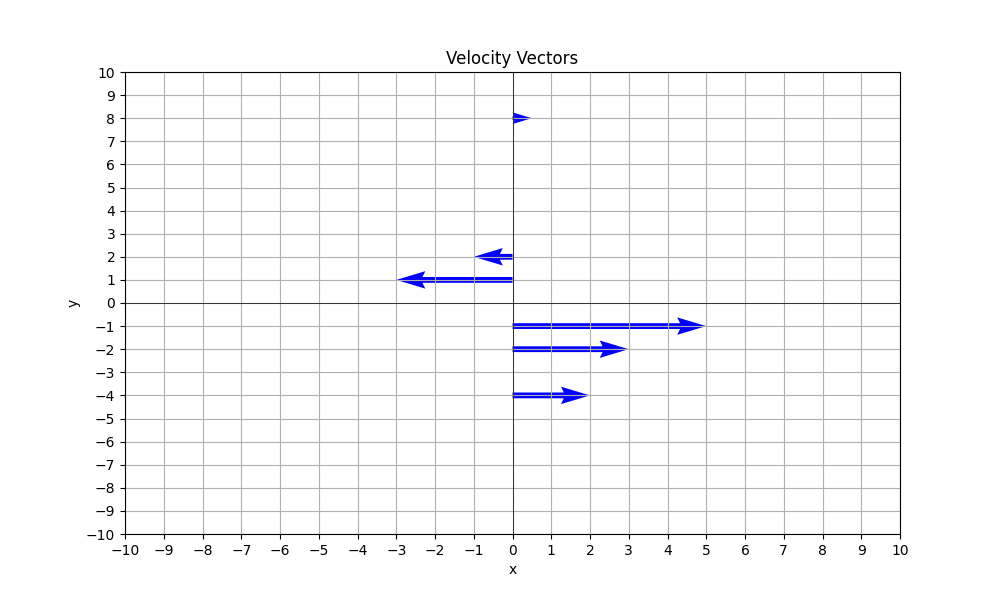
(5)
(3)とやることは同じです。
# y軸上の6点
x_values = [0, 0, 0, 0, 0, 0]
y_values = [-4, -2, -1, 1, 2, 8]

for x_value, y_value in zip(x_values, y_values):
     u_r_theta =compute_u_r_theta(x_value,y_value)
     print('(x,y)=({0},{1})でu_r={2},u_theta={3} 大きさ {4}'.format(x_value, y_value,u_r_theta[0],u_r_theta[1],u_r_theta[2]))
#出力結果
# (x,y)=(0,-4)でu_r=0,u_theta=2 大きさ 2
# (x,y)=(0,-2)でu_r=0,u_theta=3 大きさ 3
# (x,y)=(0,-1)でu_r=0,u_theta=5 大きさ 5
# (x,y)=(0,1)でu_r=0,u_theta=3 大きさ 3
# (x,y)=(0,2)でu_r=0,u_theta=1 大きさ 1
# (x,y)=(0,8)でu_r=0,u_theta=-1/2 大きさ 1/2

#リセット
u_x_values = []
u_y_values = []

for x_value, y_value in zip(x_values, y_values):
    velocity_vector_cartesian(x_value,y_value)

# グリッド間隔1でプロットを作成する
plt.figure(figsize=(10, 6))
plt.quiver(x_values, y_values, u_x_values, u_y_values, angles='xy', scale_units='xy', scale=1, color='b')
plt.xlim(-10, 10)
plt.ylim(-10, 10)
plt.axhline(0, color='black', linewidth=0.5)
plt.axvline(0, color='black', linewidth=0.5)
plt.grid(True)
plt.xticks(np.arange(-10, 11, 1))
plt.yticks(np.arange(-10, 11, 1))
plt.xlabel('x')
plt.ylabel('y')
plt.title('Velocity Vectors')
plt.show()
(6)
よって与えられた複素速度ポテンシャルは一様流れと渦糸の重ね合わせを表しています。
まとめ
pythonを使って流体力学の院試を解くことができました。
数学の問題にもチャレンジしてます↓
Discussion