東工大機械系院試をpythonで解いてみた[数学編]

はじめに

東工大の機械系の院試の問題をpythonを使って解いてみます。今回は令和3年度の数学の試験を解いていきます。過去問は以下のページにあります。
https://www.titech.ac.jp/admissions/prospective-students/admissions/past-exam-papers

問１

問1 (1)

回転体の体積を求める問題です。まず図を書いてみます。

import matplotlib.pyplot as plt
import numpy as np

#仮の値
a = 2
b = 5

# 円のパラメータ
center = (0, b)
radius = a

# 円の点を生成
theta = np.linspace(0, 2*np.pi, 100)
x = center[0] + radius * np.cos(theta)
y = center[1] + radius * np.sin(theta)

# プロット
plt.figure(figsize=(6,6))
plt.plot(x, y)
plt.plot(np.linspace(-10, 10,100), np.linspace(-10, 10,100),linestyle='--')
plt.scatter(*center, color='red', label=f'Center (0,b)')
plt.axhline(0, color='grey', linewidth=0.5)
plt.axvline(0, color='grey', linewidth=0.5)
plt.xlabel('x')
plt.ylabel('y')
plt.title('Circle and Line')
plt.xlim(-10, 10)
plt.ylim(-10, 10)
plt.xticks([])
plt.yticks([])
plt.legend(loc='upper left')
plt.show()

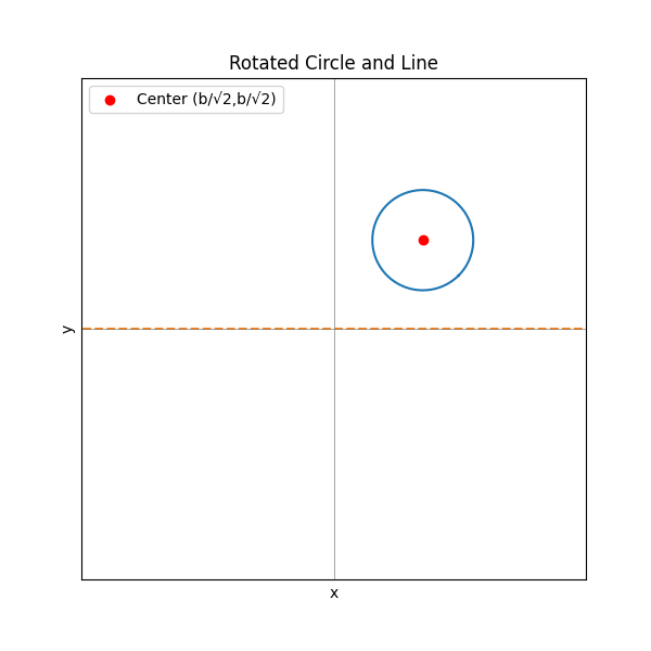
このままでは体積を求めるのは難しいので、座標を-45度回転させます。

# 座標を与えられた角度で回転させる関数
def rotate_point(x, y, angle_deg):
    angle_rad = np.radians(angle_deg)  # 角度をラジアンに変換
    x_rot = x * np.cos(angle_rad) - y * np.sin(angle_rad)  # x座標の回転
    y_rot = x * np.sin(angle_rad) + y * np.cos(angle_rad)  # y座標の回転
    return x_rot, y_rot

# y=xの直線を-45度回転させる
x_line = np.linspace(-10, 10, 100)
y_line = np.linspace(-10, 10, 100)
x_line_rot, y_line_rot = rotate_point(x_line, y_line, -45)

# 円と直線を-45度回転させる
x_rot, y_rot = rotate_point(x, y, -45)

# プロット
plt.figure(figsize=(6,6))
plt.plot(x_rot, y_rot)  # 回転した円をプロット
plt.plot(x_line_rot, y_line_rot, linestyle='--')  # 回転した直線をプロット
plt.scatter(*rotate_point(center[0], center[1], -45), color='red', label=f'Center (b/√2,b/√2)')  # 回転した円の中心をプロット
plt.axhline(0, color='grey', linewidth=0.5) 
plt.axvline(0, color='grey', linewidth=0.5) 
plt.xlabel('x')
plt.ylabel('y')
plt.title('Rotated Circle and Line')
plt.xlim(-10, 10)
plt.ylim(-10, 10)
plt.xticks([])
plt.yticks([])
plt.legend(loc='upper left')
plt.show()  

さらにx軸方向に平行移動させます。

# 回転後の新しい中心座標を計算
new_center = rotate_point(center[0], center[1], -45)

# 新しい中心のx座標を0に移動するために必要な平行移動を計算
translation_x = -new_center[0]

# 回転した円を平行移動
x_translated = x_rot + translation_x

# プロット
plt.figure(figsize=(6,6))
plt.plot(x_translated, y_rot)
plt.plot(x_line_rot, y_line_rot, linestyle='--')
plt.scatter(0, new_center[1], color='red', label=f'Center (0,b/√2)')
plt.axhline(0, color='grey', linewidth=0.5)
plt.axvline(0, color='grey', linewidth=0.5)
plt.gca().set_aspect('equal', adjustable='box')
plt.xlabel('x')
plt.ylabel('y')
plt.grid(True)
plt.title('Translated Rotated Circle and Line')
plt.xlim(-10, 10)
plt.ylim(-10, 10)
plt.xticks([])
plt.yticks([])
plt.legend(loc='upper left')
plt.show()

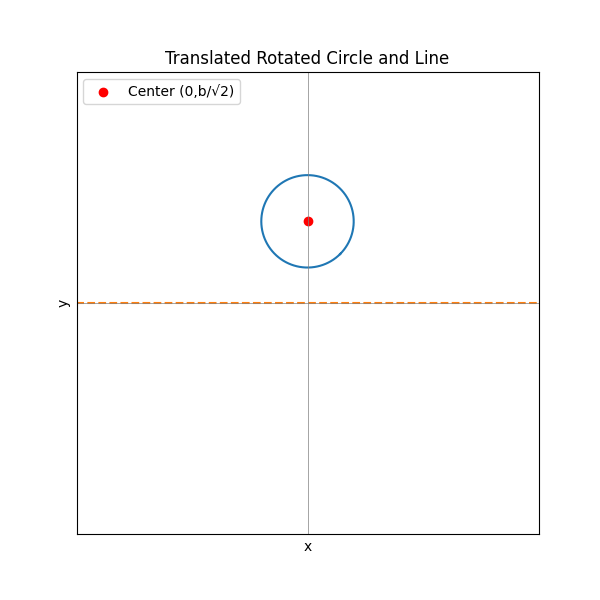
この円で囲まれた領域をx軸回りに回転させれば答えが求まります。
領域の方程式をyについて解くと、

$$y=\frac{b}{\sqrt{2}} \pm \sqrt{a^2 - x^2}$$

回転体の体積は次のように表されます。

$$V=\pi\int_{-a}^{a}(y_+^2-y_-^2)dx$$

それでは計算します。

from sympy import symbols, pi, integrate, sqrt

# 変数を定義
x = symbols('x')
a, b = symbols('a b', positive=True, real=True)

# 円盤の半径を定義
y_1= b/sqrt(2) + sqrt(a**2 - x**2)
y_2= b/sqrt(2) - sqrt(a**2 - x**2)

# 微小なスライスの体積の式を定義
dV = pi * (y_1**2 -y_2**2)

# -aからaまでの式を積分
V = integrate(dV, (x, -a, a))
V

よって答えは

$$\sqrt{2}\pi^2a^2b$$

となります。

問1 (2)

同次形の微分方程式の問題です。

from sympy import symbols, Function, Eq, diff, dsolve, tan

# 変数と関数を定義する
x, C1 = symbols('x C1')
y = Function('y')(x)
u = x + y

# 元の微分方程式 dy/dx = (x+y)^2
dy_dx_original = u**2

# u の微分方程式
du_dx = 1 + dy_dx_original

# u の微分方程式を解く
u = Function('u')(x)
differential_equation_for_u = Eq(diff(u, x), u**2 + 1)
general_solution_for_u = dsolve(differential_equation_for_u)

# y(x) に変換する
y_general_solution = general_solution_for_u.rhs - x

print('y=',y_general_solution)

答えは

$$y = -x - \tan(C_1 - x) (C_1:const)$$

となります。

問2

問2(1)

import numpy as np

# 行列Aを定義
A = np.array([[2, 1], [1, 2]])

# 固有値と固有ベクトルを計算
eigenvalues, eigenvectors = np.linalg.eig(A)

# 固有ベクトルを正規化
normalized_eigenvectors = eigenvectors / np.linalg.norm(eigenvectors, axis=0)

print(eigenvalues)#固有値
print(normalized_eigenvectors)#固有ベクトル

#出力結果
[3. 1.]
[[ 0.70710678 -0.70710678]
 [ 0.70710678  0.70710678]]

問2(2)

正則行列Pを用いて、行列Aを

$$P^{-1}AP=D$$

と対角化することで、行列Aのn乗は

$$A^n=PD^nP^{-1}$$

と求めることができます。
https://www.momoyama-usagi.com/entry/math-linear-algebra18

import numpy as np
from sympy import symbols, Matrix

# 自然数nを定義
n = symbols('n', integer=True, positive=True)

# 行列Aを定義
A = np.array([[2, 1], [1, 2]])

# Aの固有値と固有ベクトルを計算
eigenvalues, eigenvectors = np.linalg.eig(A)

# 固有ベクトルを正規化
eigenvectors = eigenvectors / np.linalg.norm(eigenvectors, axis=0)

# 行列Pを構成
P = Matrix(eigenvectors)

# 対角行列Dを構成
D = Matrix(np.diag(eigenvalues))

# Pの逆行列を計算
P_inv = P.inv()

# A^nを計算
A_n = P * D**n * P_inv
A_n

よって$A^n$は

$$\frac{1}{2} \begin{pmatrix} 3^n+1 & 3^n-1 \\ 3^n-1 & 3^n+1 \end{pmatrix}$$

となります。

問3

問3(1)

テイラー展開において、0周りでのべき級数展開を考えたものがマクローリン展開なので、

from sympy import symbols, diff, series

z = symbols('z')
f = 1/(1+z)
f_series = series(f, z, 0, 10)
f_series

答えは

$$1-z+z^2-z^3+z^4-z^5+z^6-z^7+z^8-z^9+O(z^{10})$$

となります。

問3(2)

試験ではローラン展開を行って留数を求めますが、ここでは residue 関数を使用します。

from sympy import symbols, exp, residue

z = symbols('z')
f = 1/(z*(exp(z) - 1))
res = residue(f, z, 0)
res

答えは

$$-\frac{1}{2}$$

となります。

問4

問4(1)

複素フーリエ級数$C_n$は

$$C_n=\frac{1}{T}\int_{-\frac{T}{2}}^{\frac{T}{2}}f(x)e^{-i\frac{2n\pi}{T}x}dx$$

よって

from sympy import symbols, integrate, exp, pi, I

x = symbols('x')
n = symbols('n', integer=True)

# p(x)(-0.5<=x<=0.5)を定義
p = 1

# 周期Tを定義
T = 2

# 複素フーリエ係数c_nを計算,p(x)の定義より積分範囲は(-0.5, 0.5)
c_n = (1/T) * integrate(p * exp(-I * 2*pi*n*x/T), (x, -0.5, 0.5))

# n = 0, 1, 2, 3の場合のc_nを計算
c_n_values = [c_n.subs(n, i) for i in range(4)]

# c_nの式を展開して簡単化
c_n_simplified = [c.expand(complex=True).simplify() for c in c_n_values]
c_n_simplified

答えは

$$C_0=\frac{1}{2}, C_1=\frac{1}{\pi}, C_2=0, C_3=-\frac{1}{3\pi}$$

となります。

問4(2)

パーシヴァルの等式より、

$$\int_{0}^{2}q(x)^2dx=2\sum_{n=1}^{3} C_{-n}C_n$$

$C_n$の複素共役性より、

$$2\sum_{n=1}^{3} C_{-n}C_n=2(C_{-3}^2+C_{-2}^2\cdots C_{2}^2+C_{3}^2)$$

def C(n):#(C_-3)^2から(C_3)^2まで定義
    c_n_numerical = [0.5, 1/pi, 0, -1/(3*pi)]
    return c_n_numerical[abs(n) % 4]**2
    
def sigma(func, frm, to):#Σを定義
    result = 0; 
    for i in range(frm, to+1):
        result += func(i)
    return result

ans=2*sigma(C, -3, 3)
ans   

答えは

$$\frac{9\pi^2+80}{18\pi^2}$$

となります。

まとめ

すべての問題をpythonを使って解くことができました。
既存の関数で一発で答えが出せるものもあって驚きました。