Chapter 1: What are AI Surrogate Models?
Challenges of Traditional Workflows
Traditional product design processes followed an iterative "design-simulation" workflow. This cycle can take several days per iteration. Engineers had to repeat complete physics-based simulations every time they modified a design, waiting hours for optimization results.
Here's an example using automotive fluid design:

New Workflow: Train-Predict
AWS's official solution, MLSimKit, uses machine learning to provide a new alternative to traditional workflows. The "train-predict" workflow enables predictions for new designs in minutes.

Creating a machine learning model requires a training dataset (historical input-output data from traditional workflows) and initial training time. However, once the model is built, output predictions for new CAD drawings can be made in minutes, enabling rapid design optimization.
Since the output values are predictions, you still need to perform time-consuming CAE simulations for final verification after narrowing down optimal shape candidates. However, you no longer need to iterate multiple times as with traditional methods.
This machine learning prediction model that serves as a surrogate for time-consuming, high-cost physics-based simulations is called a surrogate model.
Chapter 2: What is AI Surrogate Models in Engineering on AWS (MLSimKit)?
This is a solution included in AWS Samples (github.com/aws-samples).
About this repository:
- GitHub: AI Surrogate Models in Engineering on AWS (MLSimKit)
- License: Apache-2.0 license
- Purpose: A Python library that enables engineers to make near real-time predictions of physics-based simulations using machine learning models
This article provides a comprehensive overview of MLSimKit.
In the follow-up article:
I explain detailed procedures and results for KPI prediction of fluid simulations using AWS's AI surrogate model solution MLSimKit on EC2, targeting the WindsorML vehicle aerodynamics dataset with 210 cases. Please refer to this if you're interested.
Trial results:
• Training time: Just 14 minutes (learning from 210 cases)
• Prediction time: Just 18 seconds (testing on 70 cases)
• Prediction accuracy: MAPE 1.87% (prediction error for lift coefficient Cl - excellent)

Chapter 3: Understanding the Three Prediction Types
MLSimKit provides three different prediction types, each capturing physical phenomena at different granularities.
| Prediction Type | Example Predictions | Output Format | Architecture | Workflow |
|---|---|---|---|---|
| KPI Prediction | Integrated performance indicators (Cd, Cl, Cs, Cmy) | Numerical values (scalar) | MeshGraphNets | 4 steps (Manifest creation → Preprocessing → Training → Testing) |
| Surface Prediction | Physical quantities on surfaces (pressure, wall shear stress) | 3D mesh (.vtp) | MeshGraphNets | 4 steps (Manifest creation → Preprocessing → Training → Testing) |
| Slice Prediction | Flow fields in cross-sections (velocity, pressure) | 2D images (.png) | MeshGraphNets + AutoEncoder | 5 steps (Preprocessing+Manifest creation → Image encoder training → Mesh processing → Prediction model training → Testing) |
KPI Prediction(Key Performance Indicator Prediction)

For the entire vehicle shape, this predicts scalar values such as the drag coefficient and outputs them in CSV format.
Surface Prediction

In this example, the pressure distribution on the vehicle surface is predicted. (Note: The orientation of the drawings is reversed between input and output)
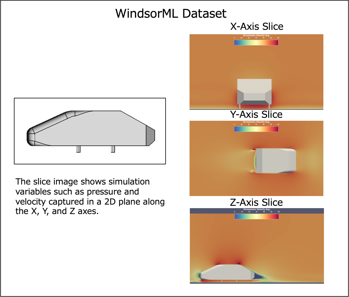
Slice Prediction

Slice prediction is used to predict parameters such as velocity and pressure from slices of 3D geometry meshes (2D cross-sections cutting through the volume, as shown in the image above).

This is a visualization of the streamwise mean velocity in cross-sections using the slice prediction model (Note: This is a different drawing from the cross-section image above).
By predicting the flow through 2D cross-sections of the 3D geometry (vehicle body) and volume (space), you can visualize the flow around the vehicle body in the cross-section.
About MGN (MeshGraphNets)
MeshGraphNet is a neural network with an Encode-Process-Decode structure (from the class docstring).
Input Data
• Node features (x): Information about each point in the mesh
• Edge features (edge_attr): Information about mesh connections
• Edge connectivity (edge_index): Which nodes are connected to each other
Processing Flow
-
Encode
• Convert node and edge features into high-dimensional vectors using MLP (Multi-Layer Perceptron) -
Process
• Repeatedly execute GraphNetBlock (process of receiving information from neighboring points and updating own information)
• Update node and edge features at each step -
Decode
• For KPI prediction as an example:
• Aggregate all node features using pooling_type (mean/max)
• Output final KPI values through a linear layer
Chapter 4: Practical Environment You Can Use Today - From Datasets to Workflows
4-1. Three Public Datasets
MLSimKit provides three public datasets hosted on Hugging Face.
Users can download large-scale pre-simulated datasets and immediately try AI surrogate models without preparing their own simulation data.
| Dataset | Total Cases | Tutorial Download Size | Features |
|---|---|---|---|
| AhmedML | 500 cases | 45GB | Basic vehicle shapes |
| WindsorML | 355 cases | 170GB | Shapes close to real vehicles |
| DrivAerML | 484 cases | 354GB | Detailed automotive models |
Common Information:
- License: All CC BY-SA 4.0
- Overview: CFD simulation collection for automotive aerodynamics modeling
Hugging Face Datasets:
- AhmedML: https://huggingface.co/datasets/neashton/ahmedml
- WindsorML: https://huggingface.co/datasets/neashton/windsorml
- DrivAerML: https://huggingface.co/datasets/neashton/drivaerml
AhmedML

Data Folder Structure
Show code (click to expand)
run_1/
├── ahmed.stl
├── boundary_1.vtp
├── force_mom_1.csv
├── force_mom_varref_1.csv
├── geo_parameters_1.csv
├── images
│   ├── CpT
│   │   ├── run_*.png
│   ├── UxMean
│   │   ├── run_*.png
├── slices
│   ├── slice_*.vtp
└── volume_1.vtu

- **ahmed_<run #>.stl** - Surface geometry definition in STL format
- **boundary_<run #>.vtp** - Surface simulation results
- **volume_<run #>.vtu** - Volume simulation output
- **force_mom_<run #>.csv** - Time-averaged force and moment coefficients
- **force_mom_varref_<run #>.csv** - Time-averaged force and moment coefficients using unique reference area per geometry
- **images** - Folder containing slice images through the volume
- **slices** - Folder containing slice vpt files rotated around x, y, z axes
WindsorML
Data Folder Structure
Show code (click to expand)
run_0/
├── boundary_0.vtu
├── force_mom_0.csv
├── force_mom_varref_0.csv
├── geo_parameters_0.csv
├── images
│   ├── pressureavg
│   │   ├── *.png
│   ├── rstress_xx
│   │   ├── *.png
│   ├── rstress_yy
│   │   ├── *.png
│   ├── rstress_zz
│   │   ├── *.png
│   ├── velocityxavg
│   │   ├── *.png
│   └── windsor_0.png
├── volume_0.vtu
├── windsor_0.stl
└── windsor_0.stp

- **windsor_<run #>.stl** - Surface geometry definition in STL format
- **boundary_<run #>.vtu** - Surface simulation results
- **volume_<run #>.vtu** - Volume simulation output
- **force_mom_<run #>.csv** - Time-averaged force and moment coefficients
- **force_mom_varref_<run #>.csv** - Time-averaged force and moment coefficients using unique reference area per geometry
- **images/** - Folder containing slice images through the volume
- **windsor_<run #>.png** - Image of Windsor body (see above)
DrivAerML

Data Folder Structure
Show code (click to expand)
run_1/
├── boundary_1.vtp
├── force_mom_1.csv
├── force_mom_constref_1.csv
├── geo_ref_i.csv
├── geo_parameters_1.csv
├── volume_1.vtu
├── drivaer_1.stl
├── images
│   ├── fig_run1_SRS_*_*Normal-*Normal-autocfd_1.png
│   ├── fig_run1_SRS_*_*Normal-*Normal_*.png
│   ├── fig_run1_SRS_iso-*.png
│   ├── fig_run1_SRS_surf-*.png
│   ├── fig_run1_SRS_*_*_grid.png
│   ├── fig_run1_evolution_*.png
│   └── fig_run1_solverStats_initialResidual.png
├── slices
│   ├── *Normal-autocfd_*.vtp
│   └── *Normal_*.vtp

- **drivaer_<run #>.stl** - Surface geometry definition in STL format
- **boundary_<run #>.vtp** - Surface simulation results
- **volume_<run #>.vtu** - Volume simulation output
- **force_mom_<run #>.csv** - Time-averaged force and moment coefficients using varying frontal area/wheelbase
- **force_mom_constref_<run #>.csv** - Time-averaged force and moment coefficients using constant frontal area/wheelbase
- **geo_ref_<run #>.csv** - Reference values for each geometry
- **geo_parameters_<run #>.csv** - Reference geometric values for each geometry
- **images/** - Folder containing images of domain slices at X, Y, Z positions (m means minus, p means plus) and various flow variables on surfaces (e.g., CpMeanTrim, kresMeanTrim, magUMeanNormTrim, microDragMeanTrim). Also includes evaluation plots for time-averaging of force coefficients (via tool MeanCalc) and residual plots showing convergence.
- **slices/** - Folder containing .vtp slices of the domain at X, Y, Z positions (m means minus, p means plus), capturing flow field variables.
4-2. Execution Workflow
4-Step Workflow (Using KPI Prediction as Example)
1. Create Manifest File
A manifest file is a JSON Lines (.jsonl) file that lists paths to data files and associated KPI values. It defines the relationship between inputs (drawings) and outputs (KPI values) in training.
-
geometry_files: List of STL or VTP file paths for a single vehicle 3D shape (CAD-designed drawing) -
kpi: List of KPI values associated with the vehicle shape (values already obtained from simulation, such as drag coefficient; optional for inference manifest)
Manifest example:
train_manifest.jsonl:
{"geometry_files": ["data/windsor/dataset/run_0/windsor_0.stl"], "kpi": [0.2818, 0.0008, 0.4882, -0.0729]}
{"geometry_files": ["data/windsor/dataset/run_1/windsor_1.stl"], "kpi": [0.2956, 0.0012, 0.5124, -0.0801]}
{"geometry_files": ["data/windsor/dataset/run_2/windsor_2.stl"], "kpi": [0.3102, -0.0005, 0.4756, -0.0688]}
...
2. Preprocess
Convert STL files to graph structures and prepare training data.
mlsimkit-learn --config config.yaml kpi preprocess \
  --manifest-file train_manifest.jsonl \
  --output-dir preprocessed-data
3. Train
Train the MeshGraphNet model and save to model-output/best_model.pth.
mlsimkit-learn --config config.yaml kpi train \
  --preprocessed-data-dir preprocessed-data \
  --output-dir model-output \
  --epochs 100
4. Test (Inference)
Predict KPI values for new shapes and output to predictions/results.csv.
mlsimkit-learn --config config.yaml kpi test \
  --manifest-file test_manifest.jsonl \
  --model-path model-output/best_model.pth \
  --output-dir predictions
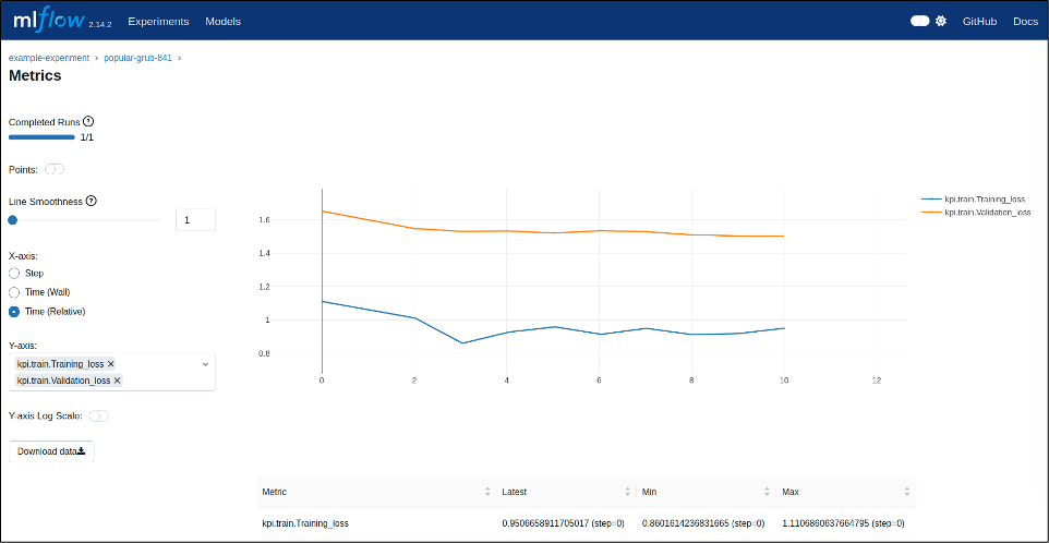
4-3. Experiment Tracking with MLflow
MLSimKit provides integration with MLflow. MLflow is an open-source platform for managing the machine learning lifecycle.
Using MLflow enables:
- Experiment tracking
- Model versioning
- Hyperparameter logging
- Metrics visualization
4-4. Execution Computing Environment
MLSimKit supports a wide range of environments, from local PC verification to practical model building on AWS cloud virtual servers (EC2).
System Requirements
Required:
• Python 3.9 or higher, below 3.13
• pip (Python package manager)

Tested Environment:
• Ubuntu 22.04 + CUDA 12.1

Other OS:
• macOS, Windows: Not officially tested, but may work as there are no OS-specific codes or dependencies (the author confirmed it works on local macOS environment)
Local Environment (For Verification)
MLSimKit includes ultra-small sample datasets that can be verified in minutes. Executable even on local PCs without GPUs.
For KPI prediction, the sample dataset contains 7 cases with a file size of several MB.
Preprocessing, training, and prediction complete in tens of seconds.
However, practical accuracy cannot be achieved due to the small number of samples.
Use cases:
• ✅ Verify MLSimKit operation
• ✅ Learn command usage
• ✅ Check output file formats
• ❌ Build practical prediction models
EC2 Environment (For Practical Use)
To build prediction models with practical accuracy, GPU-equipped EC2 instances are recommended. MLSimKit tutorials recommend AWS g5 instance family.
Recommended Environment
AMI:
• **AWS Deep Learning Base GPU AMI (Ubuntu 22.04)**
• Pre-installed with CUDA and NVIDIA
Single GPU: g5.xlarge / g5.2xlarge
Suitable instances for completing MLSimKit tutorials. Recommended for familiarizing with workflows.
g5.2xlarge specs:
• GPU: NVIDIA A10G × 1 (24GB VRAM)
• vCPU: 8 cores
• Memory: 32GB
• Cost: $1.212/hour (us-east-1)
Multi-GPU: g5.12xlarge / g5.48xlarge
After familiarizing with workflows, using multi-GPU significantly reduces training time when training on larger real-world datasets like DrivAerML.
g5.48xlarge specs:
• GPU: NVIDIA A10G × 8 (192GB VRAM total)
• vCPU: 192 cores
• Memory: 768GB
• Cost: $16.288/hour (us-east-1)
Summary
This article provided an overview of AWS's AI surrogate model solution, MLSimKit.
Traditionally, evaluating the aerodynamic performance of a single vehicle shape required hours of CFD simulation. However, using AI surrogate models enables rapid, high-accuracy prediction of aerodynamic performance for new vehicle shapes, making it possible to quickly and cost-effectively evaluate numerous shape proposals in the early design stages.
- Quantitative measurement of "rapid and high-accuracy"
Results from KPI prediction of fluid simulations on EC2 using MLSimKit with the WindsorML vehicle aerodynamics dataset of 210 cases were as follows:
• Training time: Just 14 minutes (learning from 210 cases)
• Prediction time: Just 18 seconds (testing on 70 cases)
• Prediction accuracy: MAPE 1.87% (prediction error for lift coefficient Cl - excellent)
For details, please refer to the follow-up article:

この Publication に投稿している記事は、アマゾン ウェブ サービス ジャパン合同会社または Amazon Web Services, Inc. 所属社員による個人の見解であり、所属する組織の公式見解ではありません。参加したい従業員の方は、Sugiyama Suguru までお知らせください。
Discussion