RecSys2023のTurorialを元に頻度主義A/B , ベイズA/B, Bandit A/Bについて理解する
RecSys2023のTutorial資料 を元に様々なA/Bテストについて理解する。そのメモ書き。
スライドのpdfはこちら
⚠️ メモ書きなので間違っている & 後に修正される可能性があります。
ブログで用いてる用語の説明
- variant: A, B のどちらかを表す変数
- period:a/bテスト期間内の時間単位. dataframeのrowに紐づく.
頻度主義A/B
- カイ二乗検定を用いる
chi2, p, dof, ex = hypo.chi2_test(
    n_clicks_a, N_IMPR - n_clicks_a, n_clicks_b, N_IMPR - n_clicks_b
)
print(f"chi2: {chi2:.3f}")
print(f"p-value: {p:.3f}")

# chi2: 2.411
# p-value: 0.120
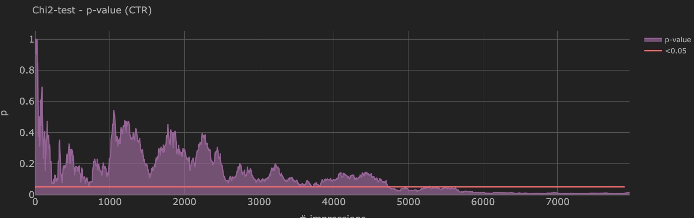
段階的にimpが発生するときのp-valueの変遷
p_data = [
    plot.plot(
        x=df.acc_impr_b,
        y=df.pvalue_ctr,
        color=1,
        opacity=0.7,
        name="p-value",
        showlegend=True,
    ),
    plot.plot(
        x=list(range(n_impressions_a)),
        y=n_impressions_a * [0.05],
        color=0,
        opacity=1,
        fill=None,
        linewidth=3,
        name="<0.05",
        showlegend=True,
    ),
]
layout = plot.layout(
    title=f"Chi2-test - p-value (CTR)",
    x_label="# impressions",
    y_label="p",
    theme="dark",
    width=1200,
    height=400,
)
fig = go.Figure(data=p_data, layout=layout).show()
- 4700impressionほどで、p-value < 0.05となる
ベイズA/Bのシミュレーションを理解する
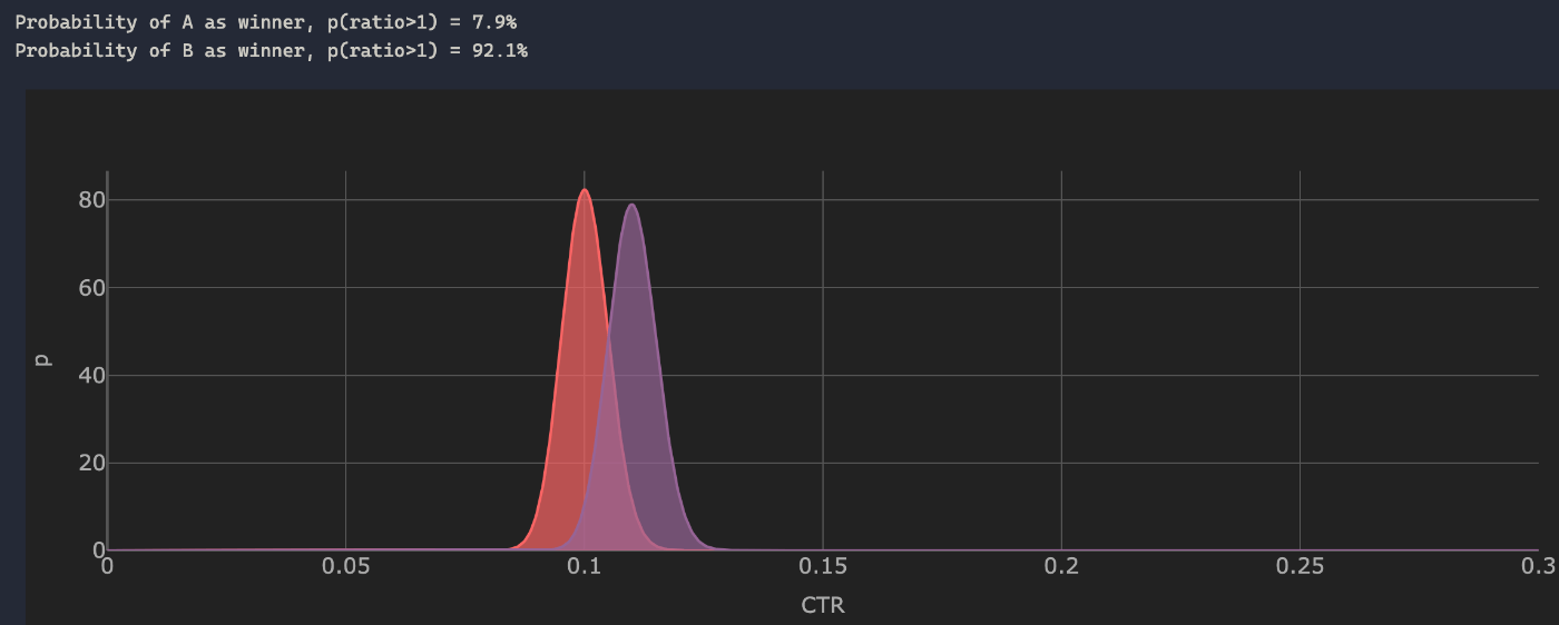
事後分布を用いた、各variantの勝率
- 2つのvariantのCTRの比較
- CTRとimpression数を既知としたときの各variantの勝率を計算する
- 事前分布はベータ分布を仮定(=共役事前分布なので、事後分布もベータ分布になる)
- パラメータは
alpha_a, beta_a = n_clicks_a + 1, N_IMPR - n_clicks_aのように計算する - 事後分布から生成した乱数を元に a/b > 1 or a/b < 1の割合を計算することで勝率を計算している
# Define Campaign Parameters
# Click-Through-Rate
CTR_A = 0.10
CTR_B = 0.11

# ---------------------------------------------------------
# Campaign simulation pararmeters
N_PERIODS = 2000 + 1
N_IMPR_PER_PERIOD = 5
SEED = 10  # both similar


# ---------------------------------------------------------
# For single evalution - number of impressons
N_IMPR = 3840  # exact # of impressions according to the hypothesis test
params = {
    "A": {"ctr": CTR_A},
    "B": {"ctr": CTR_B},
    "n_impr_per_period": N_IMPR_PER_PERIOD,
}

n_clicks_a = int(CTR_A * N_IMPR)
n_clicks_b = int(CTR_B * N_IMPR)
alpha_a, beta_a = n_clicks_a + 1, N_IMPR - n_clicks_a
alpha_b, beta_b = n_clicks_b + 1, N_IMPR - n_clicks_b

# plot CTR Beta distributions
# scan lift range
thr = 1.0
n_samples = 1_000_000
samples_a = beta.rvs(alpha_a, beta_a, size=n_samples) # random variates
samples_b = beta.rvs(alpha_b, beta_b, size=n_samples)

ratio = samples_b / samples_a # ratio of B/A
hist, bins = np.histogram(ratio, bins=1000) # histogram of ratio

# nd.array[bool]
id1, id2 = bins <= thr, bins > thr # id1: ratio <= 1, id2: ratio > 1

p_ratio_A = np.sum(hist[id1[:-1]]) / n_samples # sum of ratio <= 1 / n_samples
p_ratio_B = np.sum(hist[id2[:-1]]) / n_samples

# 事後分布(ベータ分布)における、Aの勝率とBの勝率
print(f"Probability of A as winner, p(ratio>1) = {p_ratio_A*100:.1f}%")
print(f"Probability of B as winner, p(ratio>1) = {p_ratio_B*100:.1f}%")

# ---------------------------------------------------------------------------------------------
x2 = np.linspace(0, 0.3, 1001)
p_data = [
    plot.plot(
        x=x2,
        y=beta.pdf(x2, alpha_a, beta_a), # Probability density function 確率密度分布
        color=0,
        opacity=0.7,
        name="A",
        showlegend=True,
    ),
    plot.plot(
        x=x2,
        y=beta.pdf(x2, alpha_b, beta_b),
        color=1,
        opacity=0.7,
        name="B",
        showlegend=True,
    ),
]
layout = plot.layout(
    title=f"", x_label="CTR", y_label="p", theme="dark", width=1200, height=400
)
fig = go.Figure(data=p_data, layout=layout).show()
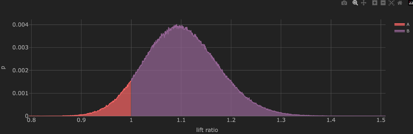
事後分布を用いた、Upliftの確率
- 事後分布の乱数からb/aの値をhistgramでplot
- treatment群によってctrがどれくらいUpliftするかを計測することができる
- 累積密度分布を計算することでuplift1.1倍になる確率は50%...などのように計算することもできる
# どれくらいUpleftするか.

p_data = [
    plot.plot(
        x=bins[id1],
        # hist: binに含まれるデータの度数(比率)
        y=hist[id1[:-1]] / sum(hist),
        color=0,
        opacity=0.7,
        name="A",
        showlegend=True,
    ),
    plot.plot(
        x=bins[id2],
        y=hist[id2[:-1]] / sum(hist),
        color=1,
        opacity=0.7,
        name="B",
        showlegend=True,
    ),
]
layout = plot.layout(
    title="", x_label="lift ratio", y_label="p", theme="dark", width=1200, height=400
)
fig = go.Figure(data=p_data, layout=layout).show()

現実に即した問題設計で、シミュレーション
- 上記のシミュレーションはすべてのimp,clickが既知の状態でのシミュレーションだった。
- 今回は徐々にimpression, clickが発生するという問題設計の元シミュレーションする
- 与えられたctrの値に即してimpression, clickを段階的に生成する
        df[f"n_impr_{variant}"] = np.random.randint(
            0, self.n_impr_per_period, n_periods
        )
        df[f"n_clicks_{variant}"] = df.apply(
            lambda x: np.random.binomial(x[f"n_impr_{variant}"], ctr), axis=1
        )
    def create(self, n_periods: int = 1000) -> pd.DataFrame:
        """Create dataframe with simulated observation stastistics for specific period

        Args:
            n_periods (int): number of simulation periods
        """
        # simulate campaign events
        df = pd.DataFrame({"t": range(n_periods)})

        # simulate impressions, clicks and costs for variants A1 / A2 / B1 / B2
        df_a1 = self.sim_impr_clicks_cost("a1", self.ctr_a, self.cpm_mean_a, n_periods)
        df_a2 = self.sim_impr_clicks_cost("a2", self.ctr_a, self.cpm_mean_a, n_periods)
        df_b1 = self.sim_impr_clicks_cost("b1", self.ctr_b, self.cpm_mean_b, n_periods)
        df_b2 = self.sim_impr_clicks_cost("b2", self.ctr_b, self.cpm_mean_b, n_periods)

        # combine all simulations into single dataframe
        df = pd.concat([df, df_a1, df_a2, df_b1, df_b2], axis=1)

        # combine A1 and A2
        df["n_impr_a"] = df.n_impr_a1 + df.n_impr_a2
        df["n_clicks_a"] = df.n_clicks_a1 + df.n_clicks_a2
        df["cost_a"] = df.cost_a1 + df.cost_a2

        # combine B1 and B2
        df["n_impr_b"] = df.n_impr_b1 + df.n_impr_b2
        df["n_clicks_b"] = df.n_clicks_b1 + df.n_clicks_b2
        df["cost_b"] = df.cost_b1 + df.cost_b2

        return df
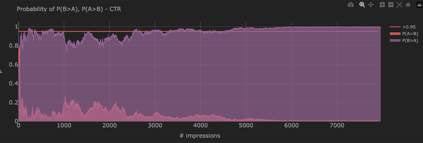
P(B>A)の変遷
- 事後分布から乱数を発生させ、P(B>A)を計算する
- 頻度主義A/Bよりかなり早くP(B>A) > 0.95になる
Bandit A/Bのシミュレーションを理解する
シミュレーションの状況理解
状況理解とBandit A/Bのモチベーション
- 広告を掲載する際に商品(もしくはクリエイティブ)A, Bどちらのほうが良いのかをA/Bテストで決めたい
- ただし通常のA/Bをすると、50%のimpressionにて、最適でない商品を露出してしまう
- どちらのほうが良いかを"探索"するのと同時に、最適な商品をなるべく多く出す"活用"も行いたい
シミュレーションの補足
- シミュレーションのためにA/Bにはそれぞれctrが事前に設定される(現実ではは未知)
- 元のコードではctrの他にcpmも計測していたが、複雑になるのでこの記事では計測していない
- 下記のようなパラメータを用いている。
- 各periodごと0~100回のimpressionが発生する(一様分布より算出)
- ctrとimpとclickがシミュレーション環境から与られ、これを元にbeta分布を仮定した事後分布のパラメータが推定される
BANDIT_PARAMS = {'A': {'period':0, 'ctr':0.1, 'cpm':1},
                  'B': {'period':0, 'ctr':0.12, 'cpm':2}}

config = {'optimise_for': 'ctr',
          'n_periods': 500,
          'max_impr_before_update_param': 100,
          'recency_param': 0.6, # decay parameter`per day`
          'n_periods_per_day': 24, # number of periods per day
          'video': 'video/bandit_abcd_ctr_slow.mp4'
         }
実装理解
Banditのトップレベルのメソッド、run()を読む。
    def run(self):
        """Run the bandit
        Iterate over all periods and update agent and environment
        Calculate metrics
        Inject new variants at specific periods
        """
        self.df_metrics = pd.DataFrame()
        for period in range(1, self.n_periods + 1):
            # ENVIRONMENT - GET IMPRESSIONS
            # random, how many impr. before updating agent
            n_impr = self.environment.simulate_impr_one_period()

            # AGENT - CHOOSE
            # ex) {'A': 35, 'B': 42}
            selected_variants = self.agent.choose(n_impr=n_impr, period=period)

            # ENVIRONMENT - RETURN CLICKS
            # ctrに基づいてimp数を元にclick数を計算する
            response = self.environment.sim_clicks_cost_one_period(selected_variants)
            print(f"period: {period} - selected_variants: {selected_variants}, response: {response}")

            # AGENT - UPDATE LOG
            log = self.agent.update_log(
                period=period,
                selected_variants=selected_variants,
                env_response=response,
            )
下記のようなフローになっている。
- periodごとに、
np.random.randint(0, config["max_impr_before_update_param"]に基づいてn_imprが計算される.- トラフィックが一定でないことを表している
- agent.chooseで各variantに割り当てられるimp数が算出される
- environment.sim_clicks_cost_one_period(selected_variants)で割り当てられたimpと事前定義されたctrからclick数が算出される
- update_logで事後分布が更新される
更に詳しく見る。
agent.choose
    def choose(self, period: int, n_impr: int) -> Union[str, int]:
        """Choose which variants to serve next
        Returns:
            selected_variants (str): names of the variant to serve
        """
        samples = {}

        # 過去の状況において、n_imprだけimpしたときに、A,Bどちらが何回勝つかを計算する
        # それは、ベータ分布からサンプリングすることで計算できる
        for variant in self.variants:
            # Get alpha and beta from previous period
            df_prev = self.df_log[variant][self.df_log[variant]["period"] == period - 1]
            # Update recency
            samples[variant] = stats.beta(a=df_prev.alpha, b=df_prev.beta).rvs(n_impr)

        # Thompson sampling
        selected_variants = np.array(
            [samples[variant] for variant in self.variants]
        ).argmax(axis=0)

        selected_variants = {
            variant: sum(self.variants[selected_variants] == variant)
            for variant in self.variants
        }
        print(f"sampled: {samples}")

        return selected_variants
samples[variant] = stats.beta(a=df_prev.alpha, b=df_prev.beta).rvs(n_impr)にて過去のperiodにおける各variantの確率分布より推定されるctrがn_imprだけ計算される。
下記の計算により、各サンプルごとに最大の値をもつvariantを計算し、それぞれのカウントを合計する。
selected_variants = np.array(
            [samples[variant] for variant in self.variants]
        ).argmax(axis=0)
update_log
    def update_log(
        self, period: int, selected_variants: Dict, env_response: Dict
    ) -> None:
        """Update log for each variant

        Args:
            period (int): current period
            selected_variants (Dict): Dictionary holding all selected variants
            env_response (Dict): Dictionary holding all environment responses

        Returns:
            log (Dict): Dictionary holding all log entries
        """
        log = {}
        # Update log for each variant
        for variant in self.variants:
            # Calc. 現在のperiodと各peridoの差分を計算
            delta = (period - self.df_log[variant]["period"]) // self.n_periods_per_day
            recency_decay = self.recency_param**delta


            # 過去のデータほど重みを小さくして、和を取る
            n_impr_w_sum = sum(self.df_log[variant]["n_impr"] * recency_decay) + 1
            n_clicks_w_sum = sum(self.df_log[variant]["n_clicks"] * recency_decay) + 1

            ctr = n_clicks_w_sum / n_impr_w_sum
            alpha = np.round(n_clicks_w_sum + 1).astype(int)
            beta = np.round(n_impr_w_sum - n_clicks_w_sum + 1).astype(int)

            scale = 1 / (n_clicks_w_sum + 1e-16)

            # Add newest raw entries to log
            tmp = {
                "period": period,
                "n_impr": selected_variants[variant],  # current impressions
                "n_impr_w_sum": n_impr_w_sum,  # accumulated weighted impressions from all previous periods
                "n_clicks": env_response[variant]["clicks"],
                "n_clicks_w_sum": n_clicks_w_sum,
                "ctr": ctr,
                # For plotting the beta & gamma distributions
                "alpha": alpha,
                "beta": beta,
                "scale": scale,
            }
            # Append as additional row to df_log
            df_tmp = pd.DataFrame(tmp, index=[0])
            self.df_log[variant] = pd.concat(
                [self.df_log[variant], df_tmp], ignore_index=True
            )

            # append to history of agents log
            log[variant] = self.df_log[variant][
                self.df_log[variant]["period"] == period
            ].to_dict(orient="records")[0]

        return log
- 各variantごとに、self.recency_paramを元に、過去のデータの重みを減衰した上で, imp数とclick数の累積和を取る
- 上記の累積和をもとに、事後分布のパラメータであるalpha, betaを計算する
- データフレームに格納し更新する
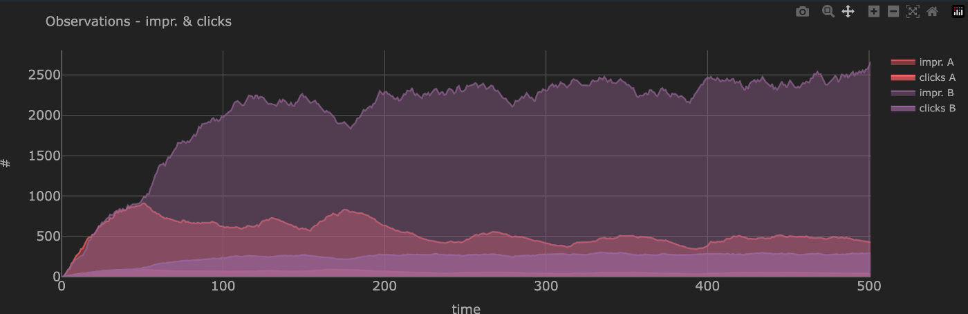
シミュレーション結果の可視化
A/Bそれぞれのimp数
click数。ctrが高いBのほうが徐々にimpが増えている。
period = 300のときのA/Bの事後分布
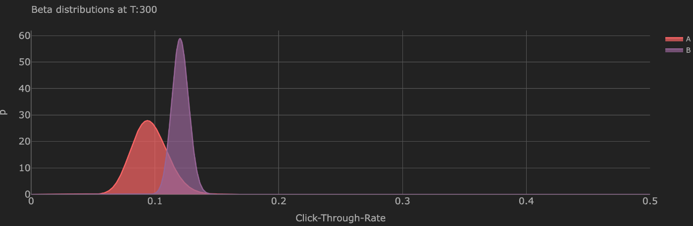
ctrが高いBのほうがログが溜まっているため、事後分布の分散が小さくなっている。
periodごとのp(A) > p(B), p(B) > (A)の確率

A/Bの事後分布から事象をサンプリングし、a/b > 1, a/b < 1となるサンプル数の割合より算出。
時刻が進むごとに p(B) > (A)の確率が高まっている
コード全体
from typing import Dict, List, Union
import numpy as np
import pandas as pd
import itertools

from scipy import stats
from scipy.stats import beta, gamma

from bayesian_test import Bayesian_AB_Test


class Environment:
    def __init__(self, env_params: Dict, config: Dict) -> None:
        self.env_params = env_params
        self.n_impr_per_period = config["max_impr_before_update_param"]

    def simulate_impr_one_period(self) -> pd.DataFrame:
        """Generate random number of impression from environment"""
        n_impr = np.random.randint(0, self.n_impr_per_period)
        return n_impr

    def simulate_clicks_one_period(self, variant: str, n_impr: int) -> pd.DataFrame:
        """Generate random clicks from environment
        Returns:
            n_clicks (int): number of clicks
        """
        n_clicks = np.random.binomial(n_impr, self.env_params[variant]["ctr"])
        return n_clicks

    def sim_clicks_cost_one_period(self, selected_variants: Dict) -> pd.DataFrame:
        """Simulate campaign observation stastistics for one period"""
        variants = list(selected_variants.keys())
        response = {}

        # Simulate impressions and clicks for all variants
        for variant in variants:
            ctr = self.env_params[variant]["ctr"]
            n_impr = selected_variants[variant]
            response.update(
                {
                    variant: {
                        "clicks": np.random.binomial(n_impr, ctr),
                    }
                }
            )

        return response


# =============================================================================
class Agent:

    def __init__(self, variants: List, config: Dict) -> None:
        """Inits class - store params locally
        """
        # Init name of variants
        self.variants = np.array(variants)

        # Init variants with zero impressions and clicks
        self.df_log = {}
        for variant in variants:
            self.create_log(variant, period=0)

        self.optimise_for = config["optimise_for"]
        self.recency_param = config["recency_param"]
        self.n_periods_per_day = config["n_periods_per_day"]

    def create_log(self, variant: str, period: int = 0) -> None:
        """Create log for agent

        Args:
            variant (str): name of the variant
            period (int): current period
        """
        self.df_log[variant] = pd.DataFrame(
            {
                "period": period,
                "n_impr": 0,
                "n_impr_w_sum": 0,
                "n_clicks": 0,
                "n_clicks_w_sum": 0,
                "ctr": 0,
                "alpha": 1,
                "beta": 1,
                "a": 1,
                "scale": 1000,
            },
            index=[0],
        )

    def update_recency(self, variant: str, period: int) -> None:
        """Update recency for each variant, both impressions and clicks
            As current timestanmpo can change, it updates all rows on only the following columns:
                - delta
                - recency
                - n_impr_w
                - n_clicks_w

        Args:
            variant (str): name of the variant
            period (int): current period

        """
        # Calc. recency
        self.df_log[variant]["delta"] = (
            period - self.df_log[variant]["period"]
        ) // self.n_periods_per_day
        self.df_log[variant]["recency"] = (
            self.recency_param ** self.df_log[variant]["delta"]
        )
        self.df_log[variant]["n_impr_w"] = (
            self.df_log[variant]["n_impr"] * self.df_log[variant]["recency"]
        )
        self.df_log[variant]["n_clicks_w"] = (
            self.df_log[variant]["n_clicks"] * self.df_log[variant]["recency"]
        )

    def choose(self, period: int, n_impr: int) -> Union[str, int]:
        """Choose which variants to serve next
        Returns:
            selected_variants (str): names of the variant to serve
        """
        samples = {}

        # 過去の状況において、n_imprしてもらったときに、A,Bどちらが何回勝つかを計算する
        # それは、ベータ分布からサンプリングすることで計算できる
        for variant in self.variants:
            # Get alpha and beta from previous period
            df_prev = self.df_log[variant][self.df_log[variant]["period"] == period - 1]
            # Update recency
            samples[variant] = stats.beta(a=df_prev.alpha, b=df_prev.beta).rvs(n_impr)

        # Thompson sampling
        selected_variants = np.array(
            [samples[variant] for variant in self.variants]
        ).argmax(axis=0)

        selected_variants = {
            variant: sum(self.variants[selected_variants] == variant)
            for variant in self.variants
        }
        print(f"sampled: {samples}")

        return selected_variants

    def update_log(
        self, period: int, selected_variants: Dict, env_response: Dict
    ) -> None:
        """Update log for each variant

        Args:
            period (int): current period
            selected_variants (Dict): Dictionary holding all selected variants
            env_response (Dict): Dictionary holding all environment responses

        Returns:
            log (Dict): Dictionary holding all log entries
        """
        log = {}
        # Update log for each variant
        for variant in self.variants:
            # Calc. 現在のperiodと各peridoの差分を計算
            delta = (period - self.df_log[variant]["period"]) // self.n_periods_per_day
            recency_decay = self.recency_param**delta


            # 過去のデータほど重みを小さくして、和を取る
            n_impr_w_sum = sum(self.df_log[variant]["n_impr"] * recency_decay) + 1
            n_clicks_w_sum = sum(self.df_log[variant]["n_clicks"] * recency_decay) + 1

            ctr = n_clicks_w_sum / n_impr_w_sum
            alpha = np.round(n_clicks_w_sum + 1).astype(int)
            beta = np.round(n_impr_w_sum - n_clicks_w_sum + 1).astype(int)

            scale = 1 / (n_clicks_w_sum + 1e-16)

            # Add newest raw entries to log
            tmp = {
                "period": period,
                "n_impr": selected_variants[variant],  # current impressions
                "n_impr_w_sum": n_impr_w_sum,  # accumulated weighted impressions from all previous periods
                "n_clicks": env_response[variant]["clicks"],
                "n_clicks_w_sum": n_clicks_w_sum,
                "ctr": ctr,
                # For plotting the beta & gamma distributions
                "alpha": alpha,
                "beta": beta,
                "scale": scale,
            }
            # Append as additional row to df_log
            df_tmp = pd.DataFrame(tmp, index=[0])
            self.df_log[variant] = pd.concat(
                [self.df_log[variant], df_tmp], ignore_index=True
            )

            # append to history of agents log
            log[variant] = self.df_log[variant][
                self.df_log[variant]["period"] == period
            ].to_dict(orient="records")[0]

        return log


# =============================================================================
class Bandit:
    """Class running the Bandit in a simulated environment"""

    def __init__(self, bandit_params: Dict, n_periods: int, config: Dict) -> None:
        self.params = bandit_params

        # Extract variants with period 0
        variants = [
            variant for variant in self.params if self.params[variant]["period"] == 0
        ]
        # Set total number of period for the experiment
        self.n_periods = n_periods
        # Extract active variant with highest ctr
        self.optimal_variant = max(
            bandit_params, key=lambda x: bandit_params[x]["ctr"] if x in variants else 0
        )

        # Init environment and agent
        self.environment = Environment(env_params=self.params, config=config)
        self.agent = Agent(variants=variants, config=config)

        # Utility functions
        self.bayes = Bayesian_AB_Test()

    def add_variant(self, variant: str, period: int, env_param: Dict) -> None:
        """Cold start - add another variant suddenly

        Args:
            variant (str): name of the variant
            period (int): current period
            env_param (Dict): Dictionary holding all environment parameters
        """
        # Add new variant to agent and log
        self.agent.variants = np.append(self.agent.variants, variant)
        self.agent.create_log(variant, period=period)
        self.environment.env_params[variant] = env_param
        self.optimal_variant = max(
            self.params,
            key=lambda x: self.params[x]["ctr"] if x in self.agent.variants else 0,
        )

    def run(self):
        """Run the bandit
        Iterate over all periods and update agent and environment
        Calculate metrics
        Inject new variants at specific periods
        """
        self.df_metrics = pd.DataFrame()
        for period in range(1, self.n_periods + 1):
            # ENVIRONMENT - GET IMPRESSIONS
            # random, how many impr. before updating agent
            n_impr = self.environment.simulate_impr_one_period()

            # AGENT - CHOOSE
            # ex) {'A': 35, 'B': 42}
            selected_variants = self.agent.choose(n_impr=n_impr, period=period)

            # ENVIRONMENT - RETURN CLICKS
            # ctrに基づいてimp数を元にclick数を計算する
            response = self.environment.sim_clicks_cost_one_period(selected_variants)
            print(f"period: {period} - selected_variants: {selected_variants}, response: {response}")

            # AGENT - UPDATE LOG
            log = self.agent.update_log(
                period=period,
                selected_variants=selected_variants,
                env_response=response,
            )

            # METRICS
            # Regret
            regret = sum(
                [
                    selected_variants[k]
                    for k in selected_variants
                    if k != self.optimal_variant
                ]
            )

            # Calc. probabilities and losses
            P_ab_ctr = self.bayes.p_ab(
                [
                    beta(log[variant]["alpha"], log[variant]["beta"])
                    for variant in self.agent.variants
                ]
            )

            loss = {"ctr": {}}
            p_overlap = {"ctr": {"ks": {}, "ws": {}}}
            for a, b in itertools.combinations(self.agent.variants, 2):
                loss["ctr"][a, b] = self.bayes.loss(
                    beta(log[a]["alpha"], log[a]["beta"]),
                    beta(log[b]["alpha"], log[b]["beta"]),
                )

            # append df_tmp to df_metrics
            df_tmp = {
                "period": period,
                "n_impr": n_impr,
                "regret": regret,
                "P_ab_ctr": [P_ab_ctr],
                "loss_ctr": [loss["ctr"]],
                "p_overlap_ctr": [p_overlap["ctr"]],
            }
            self.df_metrics = pd.concat(
                [self.df_metrics, pd.DataFrame(df_tmp, index=[0])], ignore_index=True
            )

            self.df_metrics["n_impr_acc"] = self.df_metrics["n_impr"].cumsum()
            self.df_metrics["regret_acc"] = self.df_metrics["regret"].cumsum()
            self.df_metrics["regret_avg"] = (
                self.df_metrics.regret_acc / self.df_metrics.n_impr_acc
            )

            # AGENT - cold start - add another variant suddenly
            for variant in self.params:
                if self.params[variant]["period"] == period:
                    self.add_variant(
                        variant=variant, period=period, env_param=self.params[variant]
                    )
数学的背景
だいぶ統計学や数学から遠のいていたので、かなり初歩から復習
基本用語
- 確率: 事象のおきやすさ
- 命題: 正しいか正しくないかのいずれかになる文. ex) 明日雨がフル. 猫は動物である
- 事象: 確率分布の入力となる命題。標本空間の部分集合
- p(設定 = 甘い) = 0.2
- 確率変数: 確率的に値が決まる事象. それが取る各値に対して確率が与えられている変数.
- サイコロの投げた結果を表すもの(1~6)が確率変数
- 確率分布: 命題に対してそれが生じる確率を与える対応関係.
- サイコロの各値を取る確率を示すもの
- 頻度説: 相対頻度から事象の確率を算出する. 繰り返し観測を行った時、それぞれの値がどれくらいの割合で現れるかを表すのが確率分布であるという考え方
- 台全体で甘い台の割合が全体の1/5
- 主観説・ベイズ主義: 主観的に確率を与えて分析する
- ある一つの台があった時、それが甘い台であると信じられる度合いは1/5
- ベイズ統計学: 主観確率に基づく統計分析
- 大数の法則:
- サンプルサイズが大きくなるについて、サンプル平均が母集団の平均に収束する
- = 観察された標本平均を母集団の真の平均とみなしてよい
- 中心極限定理
- 独立同分布のサンプルサイズが大きくなるについて正規分布に収束する
ベイズ基本用語
- 尤度p(x|θ):
- パラメータベクトルがθのときに観測値xの確率分布
- 観測値xに基づくθの各値のもっともらしさを表す関数.
- あるモデルの下で、観測データがどれくらい起こりやすいか
- 表が出る確率が0.5のときに、10回表が出る確率
- 最尤推定:
- 得られた観測値を得るもっともらしいθを母数と推定する行為
- 観測値が既知で母数が未知の問題設計
- 事後確率p(θ|x):
- 観測値xが与えられたときにθをがその値を取るだろうという信念の大きさ
- θがどのような値であるか、xの値を知った状態での信念の分布
- 事後確率p(θ): xが与えられる前のθをがその値を取るだろうという信念の大きさ
- 統計的推測:
- 母集団からその一部を選び出し、それを分析し、母集団について推測すること
- ハイパーパラメータ: 事前分布のパラメータのこと
- MAP推定: 事後確率を最大化するθを求める
- ベイズ推定:
- ベイズの定理を使用して、事前分布と尤度関数から事後分布を推定する
- 経験ベイズ:
- 事前分布のパラメータをデータ自体から推定する手法
- ハイパーパラメータを決めること
- ベイズ更新:
- 新しいデータが得られるたびに事後分布を更新するプロセス
ベータ分布
- 二項分布の共役事前分布
- 0と1の間の連続確率変数の確率分布
- 2つの正の形状パラメータ、α(アルファ)とβ(ベータ)をもつ
- 多項分布の共役事前分布であるディリクレ分布の次元数 = 2の場合の分布とも言える
- 尤度が二項分布で表される事象(ex. click)はa/bテストで事前分布をベータ分布とおける.
- すると、事後分布はα: 成功回数 + 1, β: 失敗回数 + 1となる
- 事前分布が何も情報がない状態を表すベータ関数(1,1)と尤度をかけることで事後分布になるから
ガンマ関数
- 実数全体で定義された階乗といえる
Thompsonサンプリング
- 確率的バンディット問題に対する解法の1つ
- 各アーム(例:A/Bテストの各バリアント)の報酬の確率分布に基づいて、アームを選択する
- 各アームの事後分布からサンプリングを行い、最も高い報酬を示すサンプルを持つアームを選択する
所感・感想
- ベイズA/Bは収束早い・途中結果がわかる・どれくらいUpliftするかなど確率で出せると言った実務上のメリットが大きい
- ただし適切な事前分布を定義するのが難しそう。例えば今回は見たい数値が0~1の正の値に限定されている
- 今回のチュートリアルは商品がA or Bの2者択一だったが、推薦のランキングでは、ユーザごとに複数のアイテムsetを出し分けるという問題設計になる。その場合でも両者の母集団の平均値(ex. CTR)を使って検定する and 同じ事前分布を用いることは妥当なのだろうか
- Bandit A/Bは探索も活用もしたい = sub-optimalなitemを長期間50%出すことが耐えられないときに便利
- 普通のA/Bは活用 = 0で探索に全振りしたe-greedyとも捉えられる
- Thompsonサンプリングを用いれば、片方が大勝しているときは早く活用に寄せるなど、自動調整できるのが便利そう
- 実装上、ベイズの事後分布を計算 → 出現割合を変化させると言ったシステムはどのレイヤーで実装するのがよいのだろうか
- Pythonレイヤでバッチ処理で計算 → 算出された固定比率を使って、Redisなどでオンラインサービング?
参考資料
なぜA/Bテストで母比率の差の検定でなく、カイ二乗検定をするのか
シミュレーションのコードを読んで、ctrの差を検定をするときに、統計検定2級で習った、母比率や母平均の差の検定でなくカイ二乗検定をしているのか気になったので調べた。

分布に差があるのかを見ているのか、平均値に差があるのかを見るかという違いがある。
ただし実利上どう使い分ければいいのかはあんまり分からなかった。
また、(ピアソンの)χ2検定は、「観察された事象の相対的頻度が、ある頻度分布に従う」 という帰無仮説を検定するものである(A/Bテストの場合、オリジナルパターンの分布と同じであるという仮説)一方、 t検定の方は(CVRなどの)平均値にA・Bパターン間で差があるかを調べるものである点が異なる。 分布を見るか、平均値を見るか、という点が異なるのである。