Linear regression model

A linear regression model is defined as follows:

$$\begin{align*} \hat{y}_n = w_0 + w_1 x_{n1} + \dots + w_D x_{nD} ,\quad w_d \in \bm{w} ,\quad x_{nd} \in \bm{x_n} , \end{align*}$$

Using matrix notation, we can express it as:

$$\begin{align*} \underbrace{ \begin{pmatrix} \hat{y}_1 \\ \hat{y}_2 \\ \vdots \\ \hat{y}_N \end{pmatrix} }_{\hat{\bm{y}}} = \underbrace{ \begin{pmatrix} 1 & x_{11} & \dots & x_{1D} \\ \vdots & & & \vdots \\ 1 & x_{N1} & \dots & x_{ND} \\ \end{pmatrix} }_{X} \underbrace{ \begin{pmatrix} w_0 \\ w_1 \\ \vdots \\ w_D \end{pmatrix} }_{\bm{w}} \end{align*}$$

$X$ is called as the design matrix of the regression model.

---

Given observations (or training data) $\mathcal{D} = \set{(x_n, y_n)}_{n=1}^N$ and the loss function $\mathcal{L}(\bm{w})$, we can obtain $\bm{w}_* = \underset{\bm{w}}{\arg\min} \mathcal{L}(\bm{w})$.

$$\begin{align*} \mathcal{L}(w) &= \sum_{n=1}^N (y_n - \hat{y}_n)^2 \\ &= \sum_{n=1}^N (y_n - \bm{w}^\top x_n)^2 \\ &= (\bm{y} - X \bm{w})^\top (\bm{y} - X \bm{w}) \\ &= \bm{y}^\top \bm{y} - 2 \bm{y}^\top X \bm{w} + \bm{w}^\top X^\top X \bm{w} \\ \frac{\partial \mathcal{L}(w) }{\partial \bm{w}} &= - 2 \bm{y}^\top X + \left( X^\top X + (X^\top X)^\top \right) \bm{w} \\ &= - 2 \bm{y}^\top X + 2 X^\top X \bm{w} \\ \end{align*}$$

By setting $\frac{\partial \mathcal{L}(w) }{\partial \bm{w}} = 0$, we can analytically solve for $\bm{w}$ using the equation $X^\top X \bm{w} = X^\top \bm{y}$. If $(X^\top X)^{-1}$ exists, we have:

$$\begin{align*} \bm{w}_* = (X^\top X)^{-1} X^\top y \end{align*}$$

---

When $(X^\top X)^{-1}$ does not exist or $\rm{rank}(X^\top X) \lt D$, $\bm{w}_*$ will be unstable.
So, we modifiy the loss function with $\alpha > 0$ as

$$\begin{align*} \mathcal{L}_{\rm{ridge}}(\bm{w}) &= (\bm{y} - X \bm{w})^\top (\bm{y} - X \bm{w}) + \alpha \| \bm{w} \|^2 \\ &= (\bm{y} - X \bm{w})^\top (\bm{y} - X \bm{w}) + \alpha \bm{w}^\top \bm{w} \\ \frac{\partial \mathcal{L}_{\rm{ridge}}(w) }{\partial \bm{w}} &= - 2 \bm{y}^\top X + 2 X^\top X \bm{w} + 2 \alpha \bm{w} , \end{align*}$$

therefore $\bm{w}_* = (X^\top X + \alpha I)^{-1} X^\top y$ .

---

If we let $A = (X^\top X + \alpha I) \in \R^{D \times D}$, $\bm{b} = (X^\top \bm{y}) \in \R^D$, then $\bm{w}_* = A^{-1} \bm{b}$, and $\bm{w}_*$ can be computed numerically stably as w = np.linalg.solve(A, b) in Python.

Here is an implementation in Python:

class LinearRegressor:
    def __init__(self, alpha=1.0e-2, intercept=True):
        self.alpha = alpha
        self.intercept = intercept
        self.w = None

    def fit(self, X, y):
        # _X : # (N, D)
        _X = np.hstack([np.ones(len(X)).reshape(-1, 1), X]) if self.intercept else X
        _, D = _X.shape

        # _y : (N, 1)
        _y = y.reshape(-1, 1) if y.ndim == 1 else y

        # w = A^{-1} b : (D, 1)
        A = (_X.T @ _X) + self.alpha * np.eye(D)  # (D, D)
        b = _X.T @ _y  # (D, 1)
        self.w = np.linalg.solve(A, b)

        return self

    def predict(self, X):
        _X = np.hstack([np.ones(len(X)).reshape(-1, 1), X]) if self.intercept else X
        return (_X @ self.w).ravel()  # (N, )

---

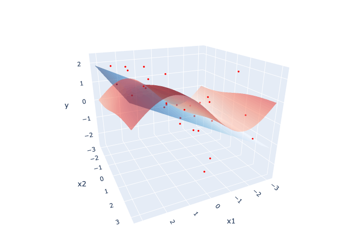
A visualization with simulated data. The true surface is colored as red, the prediction surface is colored as blue, and red points are observations (training data).

---

Data was generated as follows:

import numpy as np

## The number of data
N = 30

## The number of data dimensions
D = 2


## The true function
def f_true(X):
    return np.sin(X[:, 0]) + (1 / (1 + np.exp(-X[:, 1])))


## Observations
X = np.random.uniform(low=-np.pi, high=np.pi, size=(N, D))
y = f_true(X) + np.random.normal(scale=1.0, size=(N,))

## Build and train a model
lr = LinearRegressor(intercept=True).fit(X, y)

---

The graph was generated as follows:

#  Visualization

import plotly.graph_objects as go

## Preparation
r = np.pi
g = np.linspace(-r, r)
xx1, xx2 = np.meshgrid(g, g)
G = np.vstack([xx1.ravel(), xx2.ravel()]).T
zz = lr.predict(G).reshape(len(g), len(g))
zz_true = f_true(G).reshape(len(g), len(g))


## Plot
fig = go.Figure(
    data=[
        # Prediction surface
        go.Surface(
            x=xx1,
            y=xx2,
            z=zz,
            colorscale="Blues",
            showscale=False,
            opacity=0.5,
        ),
        # True surface
        go.Surface(
            x=xx1,
            y=xx2,
            z=zz_true,
            colorscale="Reds",
            showscale=False,
            opacity=0.5,
        ),
        # Observations
        go.Scatter3d(
            x=X[:, 0],
            y=X[:, 1],
            z=y,
            mode="markers",
            marker=dict(size=1, color="red"),
        ),
    ]
)

fig.update_layout(
    autosize=False,
    margin=dict(l=0, r=0, t=0, b=0),
    scene=dict(
        xaxis=dict(title="x1"),
        yaxis=dict(title="x2"),
        zaxis=dict(title="y"),
    ),
    showlegend=False,
)

fig.show()