【Dimensionality Reduction Method】How to use t-SNE (PCA, UMAP, DensMAP)

This time, I explain t-SNE the visual method for understanding encoded data.

1. What is the t-SNE?

t-SNE is a method of visualization of high-dimension data like vectors.

How visualize?

1. First, humans can't understand the high-dimensional data, and can't plot that. So t-SNE reduces the number of dimensions to 2-3 dimensions(e.g. from 50) for visualization.
2. But how to reduce the dimension without as much as possible missing information? t-SNE uses called "Stochastic Neighbor Embedding", this minimizes the divergence between two distributions:
   one representing pairwise similarities of the input data in the high-dimensional space and another representing pairwise similarities of the corresponding points in the low-dimensional space.

2. Advantage

・Non-Linear
Unlike PCA (Principal Component Analysis), t-SNE can capture non-linear relationships between data points.

3. Disadvantage

・Computationally Intensive
t-SNE can be slow, especially for large datasets, because it involves calculating pairwise distances and iterative optimization.
・Parameter Sensitivity
The results can be sensitive to the choice of hyperparameters, particularly the perplexity parameter which balances attention between local and global aspects of the data.
・Interpretation
While t-SNE can reveal structure in data, the exact meaning of the distances and clusters in the resulting map can be difficult to interpret.

4. Practical Use

・Perplexity
This parameter roughly corresponds to the number of nearest neighbors that are used in the manifold learning. Common values are between 5 and 50. It can affect the balance between local and global aspects of the data.

・Learning Rate
Typically, a learning rate in the range [10, 1000] is appropriate. If the cost function increases during initial optimization, the learning rate might be too high.

・Initialization
Initialization can be done using PCA (to capture the global structure) or randomly. PCA initialization often leads to better results.

・Number of Iterations
More iterations can improve the embedding, but returns diminish after a certain point. Monitoring the cost function can help decide when to stop.

When applying this to high dimensional data, I think better to reducing dimension(to about 50 or 100) by other methods like PCA before applying t-SNE.

・The reasons

1. Computational Efficiency
   t-SNE is not faster than PCA. It's efficient to apply PCA before t-SNE.

2. Noise Reduction
   High-dimensional data often contains noise and redundant information. PCA can help by capturing the most significant features and discarding the noise.

3. Improved Embeddings
   By reducing the dimensionality with PCA, t-SNE can focus on capturing the nonlinear structures in a more manageable and meaningful space, leading to better visualizations.

5. Code

import numpy as np
import matplotlib.pyplot as plt
from sklearn.manifold import TSNE
from sklearn.datasets import load_digits

# Load a sample dataset
digits = load_digits()
X = digits.data
y = digits.target

# Perform t-SNE
tsne = TSNE(n_components=2, perplexity=30, n_iter=300)
X_tsne = tsne.fit_transform(X)

# Plotting the results
plt.figure(figsize=(10, 8))
scatter = plt.scatter(X_tsne[:, 0], X_tsne[:, 1], c=y, cmap='viridis')
plt.colorbar(scatter)
plt.title('t-SNE visualization of the Digits dataset')
plt.show()

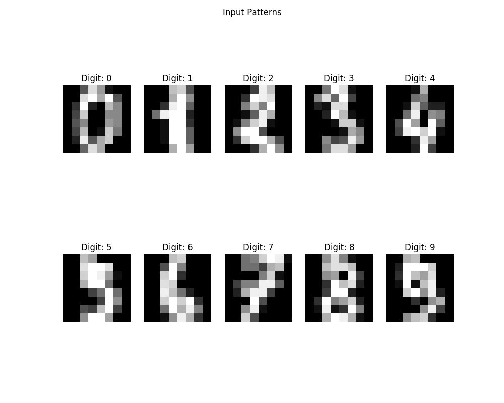
・Sample of Inputs

・Output

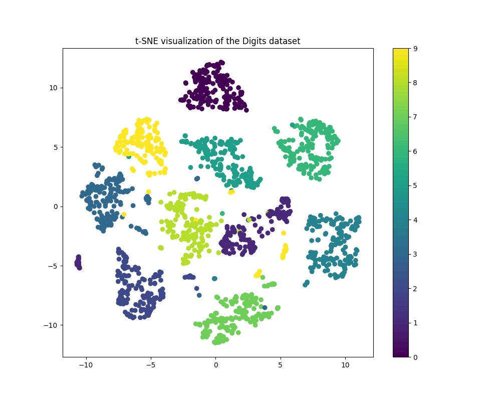
It seems t-SNE can separate the input depending on classes with good accuracy.

6. When it uses

This is useful when checking whether needs under/oversampling or not.

Applying reducing dimension methods to the embedded vector(class is a label of each data), then we can think oversampling is needed or not.
If the result shows the same label data are separated into similar vectors, and existing some groups there, it seems upsampling is valid.

In contrast, there is only one group with the correct label, upsampling doesn't perform so well. Finally, when there are no groups of correct labels, that embedding method or the data has a huge error because it indicates the embedding method embeds similar data to dissimilar vectors.

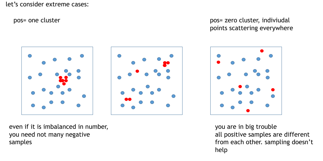
I think in the situation of the middle in the above image, oversampling may work well because there are several groups, and oversampling can reinforce the features of these groups.

7. Other methods

There are several methods for reducing the dimension, now try other methods and compare them.

・Compare methods

code

import numpy as np
import matplotlib.pyplot as plt
from sklearn.datasets import load_digits
from sklearn.decomposition import PCA
from sklearn.manifold import TSNE
import umap
import time

# Load a sample dataset
digits = load_digits()
X = digits.data
y = digits.target

# Perform PCA
start_time = time.time()
pca = PCA(n_components=2)
X_pca = pca.fit_transform(X)
pca_time = time.time() - start_time

# Perform t-SNE with PCA initialization
start_time = time.time()
tsne = TSNE(n_components=2, init='pca', perplexity=30, n_iter=300)
X_tsne_pca = tsne.fit_transform(X)
tsne_time = time.time() - start_time

# Perform UMAP
start_time = time.time()
umap_reducer = umap.UMAP(n_components=2, random_state=42)
X_umap = umap_reducer.fit_transform(X)
umap_time = time.time() - start_time

# Perform DensMAP (Densified Manifold Approximation and Projection)
start_time = time.time()
densmap_reducer = umap.UMAP(densmap=True, random_state=42)
X_densmap = densmap_reducer.fit_transform(X)
densmap_time = time.time() - start_time

# Plotting the results
plt.figure(figsize=(20, 10))

plt.subplot(2, 2, 1)
scatter![](https://storage.googleapis.com/zenn-user-upload/3ebf15dde937-20240718.png)_pca = plt.scatter(X_pca[:, 0], X_pca[:, 1], c=y, cmap='viridis', s=5)
plt.title(f'PCA (time: {pca_time:.2f} s)')
plt.colorbar(scatter_pca)

plt.subplot(2, 2, 2)
scatter_tsne_pca = plt.scatter(X_tsne_pca[:, 0], X_tsne_pca[:, 1], c=y, cmap='viridis', s=5)
plt.title(f't-SNE with PCA Initialization (time: {tsne_time:.2f} s)')
plt.colorbar(scatter_tsne_pca)

plt.subplot(2, 2, 3)
scatter_umap = plt.scatter(X_umap[:, 0], X_umap[:, 1], c=y, cmap='viridis', s=5)
plt.title(f'UMAP (time: {umap_time:.2f} s)')
plt.colorbar(scatter_umap)

plt.subplot(2, 2, 4)
scatter_densmap = plt.scatter(X_densmap[:, 0], X_densmap[:, 1], c=y, cmap='viridis', s=5)
plt.title(f'DensMAP (time: {densmap_time:.2f} s)')
plt.colorbar(scatter_densmap)

plt.tight_layout()
plt.show()

・Output

Please use the processing time as a reference because it changed a lot when I did it several times.
The trend in execution time was PCA < t-SNE <= UMAP < DensMAP.

Appendix

show input

import matplotlib.pyplot as plt
import seaborn as sns
from sklearn.datasets import load_digits

# Load the dataset
digits = load_digits()
X = digits.data
y = digits.target
images = digits.images

# Display all the input patterns
plt.figure(figsize=(10, 8))
for i in range(10):
    plt.subplot(2, 5, i + 1)
    plt.imshow(images[i], cmap='gray')
    plt.title(f'Digit: {y[i]}')
    plt.axis('off')
plt.suptitle('Input Patterns')
plt.show()

Reference