【ML】How to use the LGBM

1. LGBM

LGBM is one of the decision tree algorithms.

1.1 Advantages

Here are the advantages of LGBM. In summary, it's fast and produces good data.

1. Faster Training
   LightGBM's histogram-based algorithm and leaf-wise tree growth result in quicker training times.

2. Scalability
   It handles large datasets efficiently, including support for distributed learning.

3. Memory Efficiency
   LightGBM uses less memory due to its efficient handling of high-dimensional data and native support for categorical features.

4. Better Performance on High-dimensional Data
   It excels with datasets that have many features due to its feature bundling and efficient algorithms.

5. Customization and Flexibility
   LightGBM allows for custom loss functions and offers advanced regularization options, giving more control over the model.

1.2 Disadvantages

But, all of GBDT contains risk of overfitting.

1. Deep Trees
   If the individual trees in the GBDT are allowed to grow too deep, they become highly complex and can model intricate relationships in the training data. This complexity increases the risk of fitting noise in the data, leading to overfitting.
2. Noise Amplification
   GBDT models are sensitive to noisy data because each tree tries to correct the errors made by the previous ones. If the data contains noise, the model can start to fit this noise, resulting in a model that performs well on training data but poorly on unseen test data.

So, please be careful of overfitting. There are also some countermeasures such as the following:

• Early Stopping
  Halting the training process if the model’s performance on a validation set stops improving.
• Tree Pruning
  Limiting the depth of trees or the number of leaves to reduce model complexity.
• Regularization
  Applying regularization techniques like shrinkage (learning rate), L1/L2 regularization, and subsampling to control overfitting.

2. Code

I'll explain with code from here.

2.1 Step

1. Create Dataset
   Prepare the train and valid dataset (+test dataset)
2. Set Parameters
   Set parameters of train and configlation of model and evaluate.
3. Train
   Train the model with some hyperparameters. Please try the optimization of hyperprams by optuna(auto) or wandb(manual).
4. Predict and Postprocess
   Predict by model.predict(X_test). This time, using same dataset to valid and test, but typically, they should be separated(because using fold spilit).
   After prediction, calculate score.
5. (option) Show the Importance
   GBDT can show the importance of features. This indicate us what featture is important and we can use this information for another models like NN. This is so useful, I explain below about more detail settings.

Well, let's see the code. The below is an example code.

from sklearn.datasets import load_breast_cancer
from sklearn.model_selection import train_test_split
from sklearn.metrics import accuracy_score
import matplotlib.pyplot as plt
import pandas as pd
import lightgbm as lgb


# load the breast cancer dataset
data = load_breast_cancer()

X = data.data
y = data.target

# feature names (optional, useful for plotting and interpretation)
feature_names = data.feature_names

df = pd.DataFrame(X, columns=feature_names)
df['target'] = y
display(df.head())

# split data
X_train, X_test, y_train, y_test = train_test_split(df.drop(columns=['target']), df['target'], test_size=0.2, random_state=42)

# set params
params = {
    'objective': 'binary',               # Binary classification
    'boosting_type': 'gbdt',             # Gradient Boosting Decision Tree
    'metric': 'binary_logloss',          # Evaluation metric
    'learning_rate': 0.1,
    'num_leaves': 31,
    'verbose': -1
}

# Convert the training data into LightGBM dataset format
train_data = lgb.Dataset(X_train, label=y_train)
valid_data = lgb.Dataset(X_test, label=y_test, reference=train_data)

# Train the model with early stopping
evals_result = {}  # To record eval results for plotting
model = lgb.train(
    params,
    train_data,
    num_boost_round=100,
    valid_sets=[train_data, valid_data],
    valid_names=['train', 'valid'],
    callbacks=[lgb.record_evaluation(evals_result), lgb.early_stopping(10)],
)

# Predict probabilities
y_pred_prob = model.predict(X_test)
# Convert probabilities to binary outputs
y_pred = [1 if prob > 0.5 else 0 for prob in y_pred_prob]

accuracy = accuracy_score(y_test, y_pred)
print(f'Accuracy on test set: {accuracy * 100:.2f}%')


# Plot feature importance
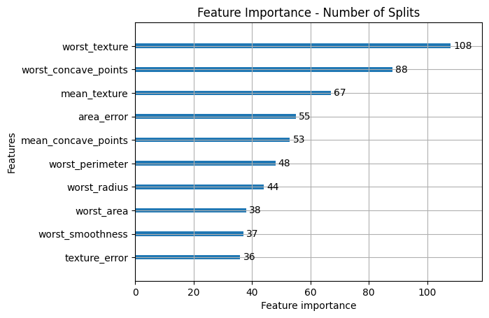
lgb.plot_importance(model, max_num_features=10, importance_type='split')
plt.title('Feature Importance - Number of Splits')
plt.show()

lgb.plot_importance(model, max_num_features=10, importance_type='gain')
plt.title('Feature Importance - Gain')
plt.show()

# Plot training log loss
plt.plot(evals_result['train']['binary_logloss'], label='train')
plt.plot(evals_result['valid']['binary_logloss'], label='valid')
plt.xlabel('Boosting Round')
plt.ylabel('Log Loss')
plt.title('Training Log Loss over Boosting Rounds')
plt.legend()
plt.show()

・Result

• table
  
• log

Training until validation scores don't improve for 10 rounds
Early stopping, best iteration is:
[45]	train's binary_logloss: 0.0202185	valid's binary_logloss: 0.10416
Accuracy on test set: 97.37%

• Importance
  If a feature is used frequently but has a low gain, it might suggest that while the feature is frequently used, it doesn't contribute much to improving the model's accuracy.
  Conversely, if a feature has a high gain but is used in fewer splits, it may indicate that while the feature is used less often, it has a significant impact when it is used.
  ・What does it mean:
  split is useful for understanding the model's decision structure—how often a feature is considered.
  gain provides a more performance-oriented view—how much a feature helps in reducing the error.
  
  
• logloss
  

3. Summary

This time, I explained about LGBM, I'm planning to write the article about another GBDT method like CatBoost and XGBoost. I'd be happy if you read that too.

Reference

[1] lightgbm.plot_importance