【For Begginer】How to use wandb (Minimum Required)

1. What is wandb

Weights and Biases (wandb) is a popular tool for experiment tracking, model management, and hyperparameter tuning in machine learning projects.

First, you go the wandb site and register, and get the api key from "User settings / Danger zone / API keys / Reveal".

2. How to use

2.1 Install

pip install wandb

2.2 Set API KEY

・Environment variable (mac/linux)

export WANDB_API_KEY=your_api_key_here

・In python code

# setting api key
wandb.login(key="your-api-key")
# if you set environment variable
# wandb.login()

# Initialize wandb
wandb.init(project="pytorch-example", name="experiment_1")

2.2 Use Example

You can track the variable log easily with wandb.log.

・Point to check

# in train loop
wandb.log({"epoch": epoch + 1, "batch": i + 1, "loss": average_loss})
# final
wandb.log({"accuracy": accuracy})

・Example Code

import torch
import torch.nn as nn
import torch.optim as optim
import torchvision
import torchvision.transforms as transforms
import wandb

# Set API key and initialize wandb with experiment name
wandb.login(key="your_api_key_here")
wandb.init(project="pytorch-example", name="experiment_1")

# Define a simple CNN model
class SimpleCNN(nn.Module):
    def __init__(self):
        super(SimpleCNN, self).__init__()
        self.conv1 = nn.Conv2d(3, 16, 3, 1)
        self.conv2 = nn.Conv2d(16, 32, 3, 1)
        self.fc1 = nn.Linear(32 * 6 * 6, 128)
        self.fc2 = nn.Linear(128, 10)

    def forward(self, x):
        x = self.conv1(x)
        x = nn.ReLU()(x)
        x = nn.MaxPool2d(2, 2)(x)
        x = self.conv2(x)
        x = nn.ReLU()(x)
        x = nn.MaxPool2d(2, 2)(x)
        x = torch.flatten(x, 1)
        x = self.fc1(x)
        x = nn.ReLU()(x)
        x = self.fc2(x)
        return x

# Load CIFAR-10 dataset
transform = transforms.Compose([transforms.ToTensor(), transforms.Normalize((0.5, 0.5, 0.5), (0.5, 0.5, 0.5))])
trainset = torchvision.datasets.CIFAR10(root='./data', train=True, download=True, transform=transform)
trainloader = torch.utils.data.DataLoader(trainset, batch_size=64, shuffle=True, num_workers=2)

testset = torchvision.datasets.CIFAR10(root='./data', train=False, download=True, transform=transform)
testloader = torch.utils.data.DataLoader(testset, batch_size=64, shuffle=False, num_workers=2)

# Initialize the model, loss function, and optimizer
model = SimpleCNN()
criterion = nn.CrossEntropyLoss()
optimizer = optim.Adam(model.parameters(), lr=0.001)

# Training loop
for epoch in range(5):  # loop over the dataset multiple times
    running_loss = 0.0
    for i, data in enumerate(trainloader, 0):
        inputs, labels = data
        optimizer.zero_grad()
        outputs = model(inputs)
        loss = criterion(outputs, labels)
        loss.backward()
        optimizer.step()

        running_loss += loss.item()
        if i % 100 == 99:  # log every 100 mini-batches
            average_loss = running_loss / 100
            print(f"[{epoch + 1}, {i + 1}] loss: {average_loss:.3f}")
            wandb.log({"epoch": epoch + 1, "batch": i + 1, "loss": average_loss})
            running_loss = 0.0

print('Finished Training')

# Save the model
PATH = './cifar_net.pth'
torch.save(model.state_dict(), PATH)

# Load the model (for evaluation)
model = SimpleCNN()
model.load_state_dict(torch.load(PATH))

# Evaluate the model
correct = 0
total = 0
with torch.no_grad():
    for data in testloader:
        images, labels = data
        outputs = model(images)
        _, predicted = torch.max(outputs.data, 1)
        total += labels.size(0)
        correct += (predicted == labels).sum().item()

accuracy = 100 * correct / total
print(f'Accuracy of the network on the 10000 test images: {accuracy:.2f}%')

# Log final accuracy
wandb.log({"accuracy": accuracy})

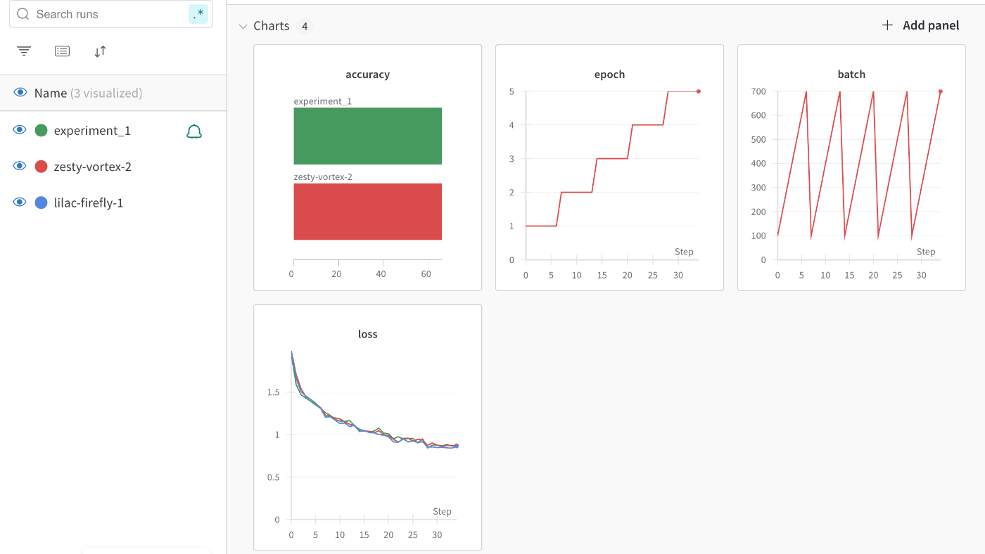
Result on wandb site

You can check the result on the wandb site. The project name is displayed on top, the experiment names are left side, and the compare graphs are shown in the middle.

Summary

This time, I introduced wandb. The experiment management tool is very useful and helps us when training models.
For example, one noticed the overfitting before 1 epoch because the test loss graph shows the minimum loss is epoch 1.

Let's use this effectively, and have a comfort development.

・Edit
Next: Hyperparameter management part is published!

Reference

[1] Weight and Biases