【ML paper】What is BBN 【Method】

1. What is BBN(Bilateral Branch Network)?

BBN is a neural network architecture conceived for handling the long-tail problem(dataset contains few classes with major data(head classes) and many classes with few data(tail classes)), it is toxic for machine learning models but a well-seen situation in the real world.

The original paper is here.

・Performances

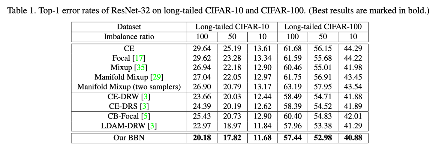
This seems to be effective for long-trailed tasks.

2. Architecture

・Architecture

BBN has two branches as itself's name. Both branches have the same residual structure from this paper and share weights without the last residual block.
There are two benefits for sharing weights:

1. the well-learned representation by the conventional
   learning branch can benefit the learning of the re-balancing
   branch.
2. sharing weights will largely reduce computational complexity in the inference phase.

I think the benefit 2 is very important in a real environment.

・Conventional Branch
This branch is designed to learn the general features of the dataset. It is trained on the entire dataset, including both head and tail classes, focusing more on the overall distribution.
・Re-balancing Branch
This branch is specifically designed to improve performance in the tail classes. It applies techniques such as re-sampling or re-weighting to give more importance to the tail classes during training.
Both re-sampling(over or under-sampling) and re-weighting(class-wise weighting or sample-wise weighting that wights minor or hard-to-predict samples with higher weights) focus on making a model that can attention to minor classes.

Finally, integrate both outputs.

・$\text{Output Fomula}$
$\bm{z} = \alpha\bm{W}_c^{\top}\bm{f}_c + (a-\alpha) \bm{W}_r^{\top}\bm{f}_r$
$\bm{z}$: output
$\alpha$: adaptive trade-off parameter
$\bm{W}$: classifier (like linear layer?)
$c, r$: Conventional Branch, Re-balancing Branch
$\bm{f}$: feature vector(output of two branches by global average pooling)

And calculate probability with softmax.
・$\text{Probability Fomula}$
$\hat{p}_i = \dfrac{e^z_i}{\sum^C_{j=1} e^z_j}$
$\hat{p}$: predicted probability
$C$: number of classes.
$i, j$: number of predictions. 0 to $C$

・$\text{Loss Function Fomula}$
$\mathcal{L} = \alpha E (\hat{\bm{p}}, y_c) + (1 - \alpha) E (\hat{\bm{p}}, y_c)$
$\mathcal{L}$: loss function
$\alpha$: coefficient
$E$: Cross entropy loss

3. Reversed sampler

Reversed sampler provides data for Re-balancing Branch.
・$\text{Sampling Fomula}$
$P_i = \dfrac{w_i}{\sum^C_{j=1} w_j}$
$\text{where} w_i = \dfrac{N_{max}}{N_i}$
$P_i$: sampling probability
$N_i$: number of samples for class i
$N_{max}$: the maximum　sample number of all the classes

Randomly sample a class according to Pi, and uniformly pick up a sample from class i with replacement. This is how to make a reversed sample dataset.

4. Cumulative learning strategy

Cumulative learning proposes the shift learning strategy. It is designed to first learn the universal patterns and then pay attention to the tail data gradually.

・$\text{Learning coefficient Fomula}$
$\alpha = 1 - (\dfrac{T}{T_{max}})^2$

$\alpha$ controls which branch affects more to model training, the bigger $\alpha$ reinforces the conventional branch's contribution to model training.
This will gradually decrease as the training epochs increase to adopt for tail classes.

5. Inference

During inference, the test samples are fed into both branches, and two features $f'_c$ and $f'_r$ are obtained. Simply fix α to 0.5 in the test phase because both branches are equally important.
Then, the equally weighted features are fed to their corresponding classifiers (i.e., $W_c$ and $W_r$) to obtain two prediction logits. Finally, both logits are aggregated by element-wise addition to return the classification results.

Reference

[1]Boyan Zhou, Quan Cui, Xiu-Shen Wei, Zhao-Min Chen, BBN: Bilateral-Branch Network with Cumulative Learning for Long-Tailed Visual Recognition, 2019
[2]Kaiming He, Xiangyu Zhang, Shaoqing Ren, and Jian Sun.
Deep residual learning for image recognition. In CVPR, pages
770–778, 2016