🐼

『Python で学ぶ衛星データ解析基礎』を R でやってみる (2) 3章後半

2025/05/12に公開

GIS

衛星データ

tech

本

前回まで

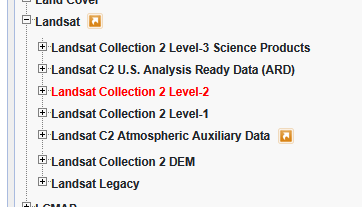
USGS Earth Explorer を利用したダウンロード方法

本では Landsat-8 の collection 1 が使われていましたが、collection 1 は現在では Earth Explorer からは選択できなくなっています。

Landsat-8 collection 2 も AWS でオープンに公開されているんですが、本で使われていた collection 1 と違って、リクエスタ支払い、つまり使う人がお金を払う設定になっています。お金を払うといっても数枚ダウンロードする程度なら 10 円もかからないでしょう。ただ、このために認証なしでは使えなくなっていて、AWS のアカウントが必要です。AWS を使い慣れていない人にはちょっとハードルがあるかもしれません。

いちおう R で S3 を使う方法を書いておくと、s3fs パッケージが便利っぽいです。request_payer = TRUE にするとリクエスタ支払いが有効にできます。ディレクトリの操作が s3_dir_*() で、ファイルの操作が s3_file_*() になっていて、まあちょっとドキュメントを読めば使えると思います。

s3fs::s3_file_system(
  profile_name = "s3-public-access",   # ~/.aws/credentials に設定している profile 名
  request_payer = TRUE,
  region_name = "us-west-2",
  refresh = TRUE
)

s3fs::s3_dir_ls("s3://usgs-landsat/collection02/")
#>  [1] "s3://usgs-landsat/collection02/catalog.json"            "s3://usgs-landsat/collection02/landsat-c2l1.json"      
#>  [3] "s3://usgs-landsat/collection02/landsat-c2l2-sr.json"    "s3://usgs-landsat/collection02/landsat-c2l2-st.json"   
#>  [5] "s3://usgs-landsat/collection02/landsat-c2l2alb-bt.json" "s3://usgs-landsat/collection02/landsat-c2l2alb-sr.json"
#>  [7] "s3://usgs-landsat/collection02/landsat-c2l2alb-st.json" "s3://usgs-landsat/collection02/landsat-c2l2alb-ta.json"
#>  [9] "s3://usgs-landsat/collection02/inventory"               "s3://usgs-landsat/collection02/level-1"                
#> [11] "s3://usgs-landsat/collection02/level-2"

本ではたぶん USGS/EROS にアカウントを作らせるのがめんどくさいということで AWS からダウンロードする方法が書かれていたんだと思いますが、USGS/EROS にアカウントをつくれば普通に Earth Explorer からダウンロードできるので、それが早いでしょう。しかもタダだし。

あるいは、前回と同じく STAC 経由でダウンロードするのもよさそうです。

stac_source <- rstac::stac("https://landsatlook.usgs.gov/stac-server")

available_collections <- stac_source |> 
  rstac::collections() |> 
  rstac::get_request()

available_collections
#> ###Collections
#> - collections (14 item(s)):
#>   - landsat-c2l2-sr
#>   - landsat-c2l2-st
#>   - landsat-c2ard-st
#>   - landsat-c2l2alb-bt
#>   - landsat-c2l3-fsca
#>   - landsat-c2ard-bt
#>   - landsat-c2l1
#>   - landsat-c2l3-ba
#>   - landsat-c2l2alb-st
#>   - landsat-c2ard-sr
#>   - landsat-c2l2alb-sr
#>   - landsat-c2l2alb-ta
#>   - landsat-c2l3-dswe
#>   - landsat-c2ard-ta
#> - field(s): collections, links, context

landsat-c2l2 というやつが collection 2（c2）の level 2（l2）らしいです。-sr となっているのが surface reflectance です。

available_collections$collections[[1]]
#> ###Collection
#> - id: landsat-c2l2-sr
#> - title: Landsat Collection 2 Level-2 UTM Surface Reflectance (SR) Product
#> - description: 
#> The Landsat Surface Reflectance (SR) product measures the fraction of incoming solar radiation that is reflected from Earth's surface to the Landsat sensor.
#> - field(s): id, type, stac_version, stac_extensions, title, description, keywords, extent, providers, license, summaries, item_assets, links

これに対して検索して、eo:cloud_cover で並べ替えます。Landsat の場合は landsat:cloud_cover_land という属性も使えそうでした（たぶん陸地の被雲率？）。

items <- stac_source |>
  rstac::stac_search(
    collections = "landsat-c2l2-sr",
    datetime = "2020-04-10T00:00:00Z/2021-06-11T00:00:00Z",
    bbox = c(139.7081, 35.4818, 139.8620, 35.6594),
    limit = 100
  ) |>
  rstac::get_request()

library(dplyr)

items |> 
  rstac::items_as_tibble() |> 
  arrange(`eo:cloud_cover`) |>
  select(datetime, `eo:cloud_cover`, `landsat:scene_id`)
#> # A tibble: 77 × 3
#>    datetime                    `eo:cloud_cover` `landsat:scene_id`   
#>    <chr>                                  <dbl> <chr>                
#>  1 2021-02-11T01:16:19.484937Z             1.8  LC81070362021042LGN00
#>  2 2020-04-29T01:15:42.798843Z             2.82 LC81070362020120LGN00
#>  3 2020-04-29T01:15:18.912039Z             2.87 LC81070352020120LGN00
#>  4 2020-11-15T00:37:43.912865Z             3    LE71070352020320ASN00
#>  5 2021-02-19T00:30:45.813798Z             4    LE71070352021050ASN00
#>  6 2020-08-11T00:44:01.557498Z             4    LE71070352020224EDC00
#>  7 2020-11-23T01:16:09.260137Z             4.62 LC81070352020328LGN00
#>  8 2021-01-10T01:16:02.819631Z             4.7  LC81070352021010LGN00
#>  9 2021-05-10T00:24:15.368007Z             6    LE71070352021130EDC00
#> 10 2021-01-02T00:34:14.847940Z             6    LE71070352021002ASN00
#> # ℹ 67 more rows
#> # ℹ Use `print(n = ...)` to see more rows

そして rstac::assets_url() でダウンロードできる URL を調べます（被雲率がいちばん低いのは LC81070362021042LGN00 でしたが、ちょっと本で使ってたのと範囲がずれていたので LC81070352020120LGN00 にしました）。

items |> 
  rstac::items_filter(filter_fn = \(x) x$properties$`landsat:scene_id` == "LC81070352020120LGN00") |> 
  rstac::assets_url(c("red", "green", "blue"))
#> [1] "https://landsatlook.usgs.gov/.../LC08_L2SP_107036_20210211_20210302_02_T1_SR_B4.TIF"
#> [2] "https://landsatlook.usgs.gov/.../LC08_L2SP_107036_20210211_20210302_02_T1_SR_B3.TIF"
#> [3] "https://landsatlook.usgs.gov/.../LC08_L2SP_107036_20210211_20210302_02_T1_SR_B2.TIF"

注意点ですが、この URL はログインが必要なものになっているので、R からダウンロードすることはできません。ブラウザで開きましょう。すでにログインしていればそのままダウンロードが開始され、ログインしていなければログイン画面が出ます。

3-2 衛星データと地上データを組み合わせる準備

（省略）

3-3 GDAL を使った衛星データ処理

まずはとりあえずプロットしてみます。ちなみに、本でキャプションに「Landsat-8 courtesy of the U.S. Geological Survey」と書かれてましたが、USGS のデータを使う時は acknowledgement の書き方が決まっているみたいです（参考）。ということでここでもそれに合わせます。

library(terra)

b5 <- rast("path/to/LC08_L2SP_107035_20200429_20200820_02_T1_SR_B5.TIF")
plot(b5)

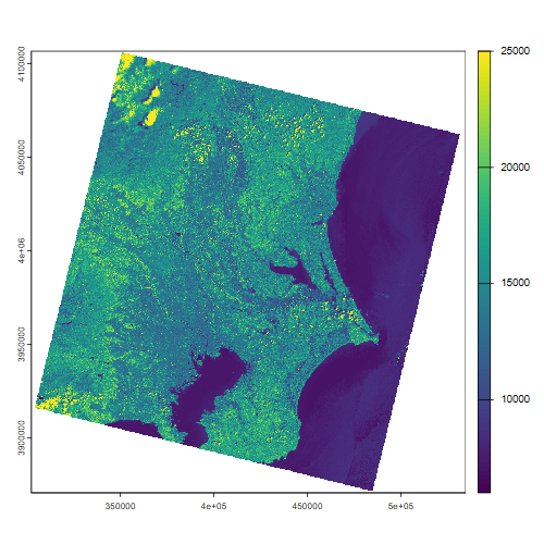
出典：Landsat-8 courtesy of the U.S. Geological Survey

値の分布の確認

値の分布を見るには hist() です。勝手にサンプリングしてやってくれるので便利。

hist(b5, breaks = 300)
#> Warning message:
#> [hist] a sample of 2% of the cells was used (of which 33% was NA)

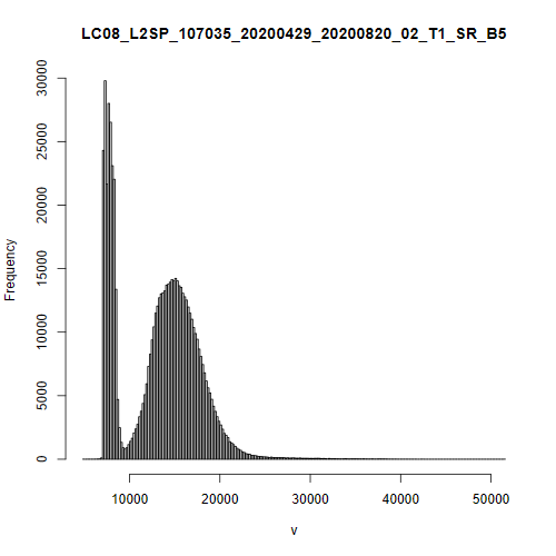
出典：Landsat-8 courtesy of the U.S. Geological Survey

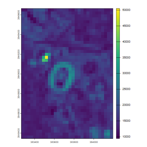
上では plot() を使いましたが、base plot でのパレットのいじり方が分からないので tidyterra パッケージを使います。パレットがいっぱいありますが、GRASS のパレットの中にある grey がグレースケールです。

# 値を 6000～25000 に絞る
b5_tweak <- b5 |>
  clamp(6000, 25000)

ggplot() +
  geom_spatraster(data = b5_tweaked) +
  scale_fill_grass_c(palette = "grey")

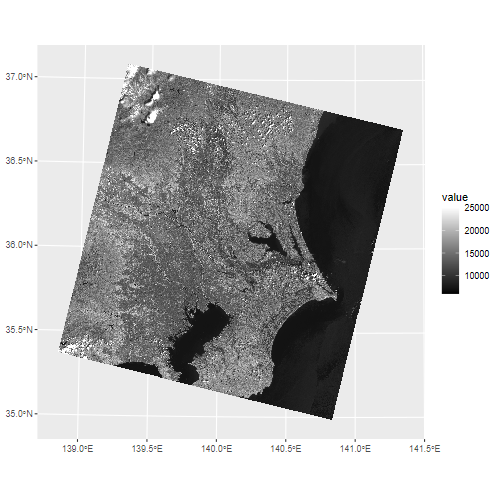
出典：Landsat-8 courtesy of the U.S. Geological Survey

3-3-3 画像の切り出し

画像の切り出しには terra::crop() を使います。ただ、本のようにピクセル単位（srcWin）で指定する方法はないみたいです。まあ別に緯度経度で指定できるし問題ないかー、と思いきや...

# xy=TRUE だと xmin, ymin, xmax, ymax の順になる
e <- ext(139.7101, 35.6721, 139.7201, 35.6841, xy = TRUE)
crop(b5, e)
#> Error:
#> ! [crop] extents do not overlap

なんと、エラーになってしまいます。よくわからないのですが、この ext() には CRS は設定できなくて、切り取り対象のラスタと同じ単位（つまりこの場合はメートル）で記述する必要があるようです。

そんなことはやってられないので、sf でポリゴンを作って投影変換して使うことにします。Geocomputation with R を見てもそうやっていたので、どうやらこれが正解っぽいです。うーん、crop() の中でいい感じに処理してほしい...^[1]

poly <- sf::st_polygon(list(
  rbind(
    c(139.7101, 35.6721),
    c(139.7201, 35.6721),
    c(139.7201, 35.6841),
    c(139.7101, 35.6841),
    c(139.7101, 35.6721)
  )
))

ext <- poly |> 
  sf::st_sfc(crs = 4326) |>   # 緯度経度として扱うために WGS84 に
  sf::st_transform(crs(b5))   # ラスタの CRS と合わせる

b5_mini <- crop(b5, ext)
plot(b5_mini)

出典：Landsat-8 courtesy of the U.S. Geological Survey

3-3-4 カラー合成

extent が揃っているラスタデータは c() で束ねられます。

b2 <- rast("path/to/LC08_L2SP_107035_20200429_20200820_02_T1_SR_B2.TIF")
b3 <- rast("path/to/LC08_L2SP_107035_20200429_20200820_02_T1_SR_B3.TIF")
b4 <- rast("path/to/LC08_L2SP_107035_20200429_20200820_02_T1_SR_B4.TIF")

rgb <- c(b4, b3, b2)

rgb
#> class       : SpatRaster 
#> dimensions  : 7871, 7741, 3  (nrow, ncol, nlyr)
#> resolution  : 30, 30  (x, y)
#> extent      : 302385, 534615, 3870585, 4106715  (xmin, xmax, ymin, ymax)
#> coord. ref. : WGS 84 / UTM zone 54N (EPSG:32654) 
#> sources     : LC08_L2SP_107035_20200429_20200820_02_T1_SR_B4.TIF  
#>               LC08_L2SP_107035_20200429_20200820_02_T1_SR_B3.TIF  
#>               LC08_L2SP_107035_20200429_20200820_02_T1_SR_B2.TIF  
#> names       : LC08_L2SP_~2_T1_SR_B4, LC08_L2SP_~2_T1_SR_B3, LC08_L2SP_~2_T1_SR_B2

トゥルーカラーでプロットするには、plotRGB() が使えます。この関数が受け付けるのは 0～255 の範囲の値なので、streatch() を指定して修正します。minvとmaxvはデフォルトの値と同じなので指定しなくて大丈夫ですが、ここでは説明のために書いています。以降は省略します。

rgb |> 
  crop(ext) |> 
  stretch(
    smin = 7000, smax = 13500,  # 入力の値の範囲
    minv = 0,    maxv = 255     # 出力される値の範囲（デフォルトの値）
  ) |> 
  plotRGB()

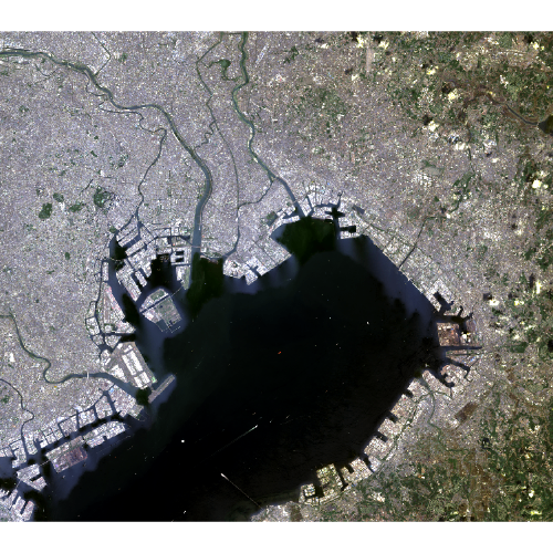
出典：Landsat-8 courtesy of the U.S. Geological Survey

smin、smax で直接値の範囲を指定するのではなく、minq、maxq でパーセンタイルを指定することもできます。例えば、上下5%を切り捨てるにはこんな感じです。

stretch(rgb, minq = 0.05, maxq = 0.95)

本でやっているように、バンドごとに値のスケールを調整してから束ねる場合はこんな感じのはずです（が、なんかこのデータの場合は見た目はイマイチでした。範囲を変える必要がある...？）。

rgb <- c(
  b4 |> crop(ext) |> stretch(smin = 7000, smax = 13000),
  b3 |> crop(ext) |> stretch(smin = 8100, smax = 12800),
  b2 |> crop(ext) |> stretch(smin = 9700, smax = 13400)
)

plotRGB(rgb)

また、tidyterra の場合は geom_spatraster_rgb() という Geom が用意されています。plotRGB() も geom_spatraster_rgb() も、どのレイヤーを赤緑青のどれに割り当てるかを選ぶことができるので、今度はそのやり方でやってみます。

# まずは全部一つに束ねる
data <- c(b2, b3, b4, b5) |> 
  crop(ext) |> 
  stretch(minq = 0.05, maxq = 0.95)

do_plot <- function(r, g, b, title) {
  ggplot() +
    # 赤緑青それぞれの割り当てを r, g, b で指定する
    tidyterra::geom_spatraster_rgb(data = data, r = r, g = g, b = b) +
    ggtitle(title)
}


patchwork::wrap_plots(
  do_plot(3, 2, 1, "True Color"),
  do_plot(4, 3, 2, "False Color"),
  do_plot(3, 4, 2, "Natural Color"),
  nrow = 2
)

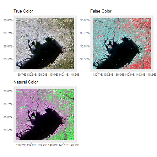
出典：Landsat-8 courtesy of the U.S. Geological Survey

3-3-5 パンシャープン画像の作成

パンシャープニングは、RStoolbox というパッケージの panSharpen() を使うとできるみたいです。

まずはデータの取得です。バンド8は level 2 ではなく level 1 にあるので、landsat-c2l1 を検索しなおします。scene_id は先ほど指定したものと同じです。

items <- stac_source |>
  rstac::stac_search(
    collections = "landsat-c2l1",
    datetime = "2020-04-10T00:00:00Z/2020-06-11T00:00:00Z",
    bbox = c(139.7081, 35.4818, 139.8620, 35.6594),
    limit = 100
  ) |>
  rstac::get_request()

items |> 
  rstac::items_filter(filter_fn = \(x) x$properties$`landsat:scene_id` == "LC81070352020120LGN00") |> 
  rstac::assets_url("pan")
#> [1] "https://.../LC08_L1TP_107035_20200429_20200820_02_T1_B8.TIF"

ダウンロードしたら、これを使って panSharpen() を使います。

pan <- rast("path/to/LC08_L1TP_107035_20200429_20200820_02_T1_B8.TIF")

# ディズニーランド周辺
poly <- sf::st_polygon(list(
  rbind(
    c(139.8697, 35.6403),
    c(139.8971, 35.6403),
    c(139.8971, 35.6212),
    c(139.8697, 35.6212),
    c(139.8697, 35.6403)
  )
))
ext <- poly |> 
  sf::st_sfc(crs = 4326) |> 
  sf::st_transform(crs(b2))

# 重いのでまず crop しておく
orig <- c(b4, b3, b2) |> crop(ext)
pan <- pan |> crop(ext)

pansharpened <- panSharpen(orig, pan, r = 1, g = 2, b = 3)

結果です。なんかくっきりしている気がします。

p1 <- ggplot() +
  tidyterra::geom_spatraster_rgb(data = stretch(orig, maxq = 0.95)) +
  ggtitle("Original")

p2 <- ggplot() +
  tidyterra::geom_spatraster_rgb(data = stretch(pansharpened, maxq = 0.95)) +
  ggtitle("After")

patchwork::wrap_plots(p1, p2)

出典：Landsat-8 courtesy of the U.S. Geological Survey

続き

脚注

stars::st_crop() の方がどう見ても使いやすそう... ↩︎

本

前回まで

USGS Earth Explorer を利用したダウンロード方法

3-2 衛星データと地上データを組み合わせる準備

3-3 GDAL を使った衛星データ処理

値の分布の確認

3-3-3 画像の切り出し

3-3-4 カラー合成

3-3-5 パンシャープン画像の作成

続き

Discussion