【Python】実践データ分析100本ノック 第1章
この記事は、現場で即戦力として活躍することを目指して作られた現場のデータ分析の実践書である「Python 実践データ分析 100本ノック(秀和システム社)」で学んだことをまとめています。
ただし、本を参考にして自分なりに構成などを変更している部分が多々あるため、ご注意ください。細かい解説などは是非本をお手に取って読まれてください。

【リンク紹介】
・【一覧】Python実践データ分析100本ノック
・これまで書いたシリーズ記事一覧
目的
ある企業のECサイトでの商品の注文数の推移を分析することによって、売上改善の方向性を探る。
Import
%%time

import pandas as pd
from colorama import Fore, Style, init                # Pythonの文字色指定ライブラリ
from IPython.display import display_html, clear_output
from gc import collect                                # ガーベッジコレクション
import matplotlib.pyplot as plt
%matplotlib inline
%%time

# テキスト出力の設定
def PrintColor(text:str, color = Fore.GREEN, style = Style.BRIGHT):
    print(style + color + text + Style.RESET_ALL);

# displayの表示設定
pd.set_option('display.max_columns', 50);
pd.set_option('display.max_rows', 50);

print()
collect()
Knock1:データの読み込み
必要なデータを読み込んでいきます。
なお、テキストのデータダウンロードは以下に格納されています。
https://www.shuwasystem.co.jp/support/7980html/6727.html
ここでは第1章で用いるデータをまとめて読み込んでいるため、テキストとは大きく異なるのでご注意ください。
%%time

# 保存先は各自の保存先を参照してください。
customer_master      = pd.read_csv('customer_master.csv')
item_master          = pd.read_csv('item_master.csv')
transaction_1        = pd.read_csv('transaction_1.csv')
transaction_2        = pd.read_csv('transaction_2.csv')
transaction_detail_1 = pd.read_csv('transaction_detail_1.csv')
transaction_detail_2 = pd.read_csv('transaction_detail_2.csv')

print()
collect()
読み込んだデータを表示してみます。
%%time

PrintColor(f'\n customer_master')
display(customer_master.head())

PrintColor(f'\n item_master')
display(item_master.head())

PrintColor(f'\n transaction_1')
display(transaction_1.head())

PrintColor(f'\n transaction_2')
display(transaction_2.head())

PrintColor(f'\n transaction_detail_1')
display(transaction_detail_1.head())

PrintColor(f'\n transaction_detail_2')
display(transaction_detail_2.head())

print()
collect()
Knock2:データを結合する(行方向に結合)
transaction_1とtransaction_2を、transaction_detail_1とtransaction_detail_2を
それぞれ行方向に結合します。
%%time

transaction        = pd.concat([transaction_1, transaction_2],
                               ignore_index = True              # 結合時にラベルが振り直される
                              )
transaction_detail = pd.concat([transaction_detail_1, transaction_detail_2],
                               ignore_index = True
                              )

print()
collect()
結合したデータを表示してみましょう(といっても、最初の5行のみ表示してるのでぱっと見は変化がありません。)
%%time

# データを表示する
PrintColor(f'\n transaction')
display(transaction.head())

PrintColor(f'\n transaction_detail')
display(transaction_detail.head())

print()
collect()
Knock3:売上データ同士を結合する
transaction_detailにtransactionのpayment_date列とcustomer_id列のデータを付与します。
%%time

join_data = pd.merge(transaction_detail,
                     transaction[['transaction_id', 'payment_date', 'customer_id']],
                     on  = 'transaction_id',   # transaction_idをキーと指定。これでtransaction_idに対応したデータを紐づけできる
                     how = 'left'              # 左結合
                    )

print()
collect()
付与後のデータを表示してみます。
%%time

# データを表示する
PrintColor(f'\n join_data')
display(join_data.head())

print()
collect()
次に、データ件数を確認してみます。
これにより、データ付与後もインデックス数は増えていないことがわかると思います。
%%time

PrintColor(f'\n transaction_detail')
print(len(transaction_detail))

PrintColor(f'\n transaction')
print((len(transaction)))

PrintColor(f'\n join_data')
print(len(join_data))

print()
collect()
Knock4:マスターデータを結合する
join_dataにcustomer_masterとitem_masterのデータを付与します。
# customer_masterを付与する
join_data = pd.merge(join_data,
                     customer_master,
                     on  = 'customer_id',
                     how = 'left'
                    )

# item_master
join_data = pd.merge(join_data,
                     item_master,
                     on  = 'item_id',
                     how = 'left'
                    )
付与した後のデータを確認します。
%%time

PrintColor(f'\n join_data')
display(join_data)

print()
collect()
Knock5:必要なデータ列を作る
quantity列とitem_price列を用いて売上列を作成します。
%%time

join_data['price'] = join_data['quantity'] * join_data['item_price']

print()
collect()
作成したデータを確認します。
%%time

PrintColor(f'\n join_data')
display(join_data[['quantity', 'item_price', 'price']].head())

print()
collect()
Knock6:データ検算をする
ptice合計値を確認していきます。
%%time

PrintColor(f"\n join_data['price']")
display(join_data['price'].sum())

PrintColor(f"\n transaction['price']")
display(transaction['price'].sum())

# もしくは以下の方法でも確認可能
PrintColor(f"\n join_data['price'].sum() == transaction['price'].sum()")
print(join_data['price'].sum() == transaction['price'].sum())

print()
collect()
Knock7:各統計量を把握する
まず、欠損値の数を出力します。
%%time

join_data.isnull().sum()
次に、基本統計量を出力します。
%%time

join_data.describe()
現在扱っているデータの期間範囲を確認しておきます。
%%time

PrintColor(f"\n join_data['payment_date'].min()")
display(join_data['payment_date'].min())

PrintColor(f"\n join_data['payment_date'].max()")
display(join_data['payment_date'].max())

print()
collect()
Knock8:月別でpriceデータを集計する
まず、データ型を確認します。
%%time

join_data.dtypes
payment_dateについて、object型からdatetime型に変換します。
%%time

join_data['payment_date'] = pd.to_datetime(join_data['payment_date'])

print()
collect()
次に、年月列を作成します。
%%time

join_data['payment_month'] = join_data['payment_date'].dt.strftime('%Y%m')

print()
collect()
[memo]
strftime() : str + f(format) + time. datetime型を指定したフォーマットの文字列に変換するメソッド
作成したデータを確認します。
%%time

PrintColor(f"\n join_data[['payment_date', 'payment_month']]")
display(join_data[['payment_date', 'payment_month']].head())

print()
collect()
最後に、月別でpriceデータを集計する。
%%time

# テキストだと['price']と.sum()の位置が逆。誤植?
join_data.groupby('payment_month')['price'].sum()
Knock9:月別、商品別でデータを集計する
%%time
join_data.groupby(['payment_month', 'item_name'])[['price', 'quantity']].sum()
作成したデータを、今度はpivot_tableを用いて表示する。
%%time

# pivot_tableを使用して集計を行う
pd.pivot_table(join_data,
               index   = 'item_name',
               columns = 'payment_month',
               values  = ['price', 'quantity'],
               aggfunc = 'sum'
              )
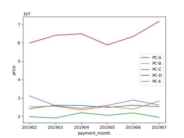
Knock10:商品別の売上推移を可視化する
商品別の月ごとの売上データを作成します。
%%time

graph_data = pd.pivot_table(join_data,
                            index   = 'payment_month',
                            columns = 'item_name',
                            values  = 'price',
                            aggfunc = 'sum'
                           )

print()
collect()
データを確認します。
%%time

PrintColor(f'\n graph_data')
display(graph_data.head())

print()
collect()
graph_dataを用いて売上推移を描画します。
%%time

plt.plot(list(graph_data.index), graph_data['PC-A'], label = 'PC-A')
plt.plot(list(graph_data.index), graph_data['PC-B'], label = 'PC-B')
plt.plot(list(graph_data.index), graph_data['PC-C'], label = 'PC-C')
plt.plot(list(graph_data.index), graph_data['PC-E'], label = 'PC-D')
plt.plot(list(graph_data.index), graph_data['PC-D'], label = 'PC-E')

# 軸ラベルの設定
plt.ylabel('price')
plt.xlabel('payment_month')
# 凡例を表示
plt.legend()

print()
collect()
ご協力のほどよろしくお願いします。
Discussion