【Python】実践データ分析100本ノック 第5章
この記事は、現場で即戦力として活躍することを目指して作られた現場のデータ分析の実践書である「Python 実践データ分析 100本ノック(秀和システム社)」で学んだことをまとめています。
ただし、本を参考にして自分なりに構成などを変更している部分が多々あるため、ご注意ください。細かい解説などは是非本をお手に取って読まれてください。

【リンク紹介】
・【一覧】Python実践データ分析100本ノック
・これまで書いたシリーズ記事一覧
目的
第3章、第4章で扱ったスポーツジムの会員の行動情報を用いて、顧客が退会してしまうのかを予測する流れを学ぶ
Import
# 必要に応じてインストールを行う
#!pip install japanize_matplotlib > /dev/null    # matplotlibで日本語表示を行う
%%time

import pandas as pd
from colorama import Fore, Style, init                # Pythonの文字色指定ライブラリ
from IPython.display import display_html, clear_output
from gc import collect                                # ガーベッジコレクション
import matplotlib.pyplot as plt
%matplotlib inline

from dateutil.relativedelta import relativedelta      # 日付に月単位で計算をする
from sklearn.tree import DecisionTreeClassifier
import sklearn.model_selection
from sklearn import tree
import matplotlib.pyplot as plt
import japanize_matplotlib
%matplotlib inline
%%time

# テキスト出力の設定
def PrintColor(text:str, color = Fore.GREEN, style = Style.BRIGHT):
    print(style + color + text + Style.RESET_ALL);

# displayの表示設定
pd.set_option('display.max_columns', 50);
pd.set_option('display.max_rows', 50);

print()
collect()
Knock41:データを読み込んで利用データを整形する
必要なデータを読み込んでいきます。
なお、テキストのデータダウンロードは以下に格納されています。
%%time

customer      = pd.read_csv('customer_join.csv')
uselog_months = pd.read_csv('use_log_months.csv')

print()
collect()
%%time

# 確認用
PrintColor(f'\n customer')
display(customer.head())

PrintColor(f'\n uselog_months')
display(uselog_months.head())

print()
collect()
次に機械学習用に利用データを加工します。
当月と1か月前のデータの利用履歴(利用回数)のみのデータを作成します。Knock36と同様の方法で処理を行います。
%%time

year_months = list(uselog_months['年月'].unique())

# 確認用
PrintColor(f'\n year_months')
display(year_months)

print()
collect()
%%time

# 格納用のDataFrameを作成
uselog      = pd.DataFrame()

# 2018年5月以降の月を一つずつ取り出す。当月と「1ヶ月前」のデータが必要なため、2018年4月は入らない。
for i in range(1, len(year_months)):
    # year_monthsリストのi番目と等しい年月をtmpに格納する
    tmp = uselog_months.loc[uselog_months['年月'] == year_months[i]].copy()
    # tmpに格納した年月を当月として考え、その利用回数名(count)をcount_0と名前を変更する
    tmp.rename(columns = {'count' : 'count_0'}, inplace = True)
    # 1ヶ月前の利用回数をtmp_beforeに格納する
    tmp_before = uselog_months.loc[uselog_months['年月'] == year_months[i - 1]].copy()

    del tmp_before['年月']

    # 名前をcount_1とする
    tmp_before.rename(columns = {'count' : 'count_1'}, inplace = True)
    # 横方向に結合し、列を追加する
    tmp = pd.merge(tmp,
                   tmp_before,
                   on  = 'customer_id',
                   how = 'left'
                  )

    # 集計が済むたびに縦に結合する
    uselog = pd.concat([uselog, tmp], ignore_index = True)

print()
collect()
%%time

PrintColor(f'\n uselog')
display(uselog.head())

print()
collect()
Knock42:退会前月の退会顧客データを作成する
退会「前」月を作成します。あくまで目的は退会を未然に防ぐことだからです。
%%time

exit_customer = customer.loc[customer['is_deleted'] == 1].copy()
# 退会「前」月を格納するカラムを作成
exit_customer['exit_date'] = 0            # テキストはNoneを指定しているが、Knock28と同様に0で初期化した
# 退会月をobject型からdatetime型へ変換する
exit_customer['end_date']  = pd.to_datetime(exit_customer['end_date'])

for i in exit_customer.index:
    exit_customer.loc[i, 'exit_date'] = exit_customer.loc[i, 'end_date'] - relativedelta(months = 1) # month = 1としないように注意

# 列の追加
exit_customer['exit_date'] = pd.to_datetime(exit_customer['exit_date'])
exit_customer['年月']      = exit_customer['exit_date'].dt.strftime('%Y%m')
uselog['年月']             = uselog['年月'].astype(str)

exit_uselog = pd.merge(uselog,
                       exit_customer,
                       on  = ['customer_id', '年月'],
                       how = 'left'
                      )

print()
collect()
[memo]
relativedelta(months = 1) ⇒ 1ヶ月分を加算する
relativedelta(month = 1) ⇒ 加算するのではなく月を1月に書き換える
参考資料:「Pythonで日付の加算、特にnヶ月後やn年後の日付を求める方法」 by YOUTAROさん
%%time

# データの確認
PrintColor(f'\n len(uselog)')
display(len(uselog))

PrintColor(f'\n exit_uselog')
display(exit_uselog.head())

print()
collect()
欠損値のあるデータは除外します。
%%time

exit_uselog = exit_uselog.dropna(subset = ['name'])

PrintColor(f'\n len(exit_uselog)')
print(len(exit_uselog))

PrintColor(f"\n len(exit_uselog['customer_id'].unique())")
print(len(exit_uselog['customer_id'].unique()))

PrintColor(f'\n exit_uselog')
display(exit_uselog.head())

print()
collect()
Knock43:継続顧客のデータを作成する
継続顧客は退会月がないため、どの年月のデータを作成してもよいです。
%%time

# is_deleted列が0(=まだ継続している)のデータのみを格納する
conti_customer = customer.loc[customer['is_deleted'] == 0]
# 結合して列を追加
conti_uselog   = pd.merge(uselog,
                          conti_customer,
                          on  = ['customer_id'],
                          how = 'left'
                         )


# 確認用
PrintColor(f'\n before len(conti_uselog)')
print(len(conti_uselog))

# 名前が欠損しているデータを除去する
conti_uselog = conti_uselog.dropna(subset = ['name'])

# 確認用
PrintColor(f'\n after len(conti_uselog)')
print(len(conti_uselog))

print()
collect()
退会データが1104件に対し、継続顧客データが27422件で約24倍もの差がある不均衡データであるため、アンダーサンプリングを行い、継続顧客データを退会データの件数に合わせていきます。
%%time

"""アンダーサンプリングを行う → 顧客データ当たり1件になるように重複データを削除する"""

# まずはデータをシャッフルする
conti_uselog = conti_uselog.sample(frac = 1, random_state = 0).reset_index(drop = True)
# customer_idの重複データを取り除く
conti_uselog = conti_uselog.drop_duplicates(subset = 'customer_id')

# 確認用
PrintColor(f'\n len(conti_uselog)')
display(len(conti_uselog))

PrintColor(f'\n conti_uselog')
display(conti_uselog.head())

print()
collect()
退会データと継続顧客データのバランスが改善されたので、2つのデータを結合していきます。
%%time

predict_data = pd.concat([conti_uselog, exit_uselog], ignore_index = True)

# 確認用
PrintColor(f'\n len(predict_data)')
print(len(predict_data))

PrintColor(f'\n predict_data')
display(predict_data.head())

print()
collect()
Knock44:予測する月の在籍期間を作成する
第4章と同じように在籍期間の列を追加します。
%%time

# now_date列を作成してdatetime型の'年月'列の値(%Y%m)で初期化する
predict_data['now_date']   = pd.to_datetime(predict_data['年月'], format = '%Y%m')
# start_date列を作成してdatetime型のstart_date列の値で初期化する
predict_data['start_date'] = pd.to_datetime(predict_data['start_date'])

predict_data['period'] = 0

for i in range(len(predict_data)):
    # 加入年月から現在までの在籍期間を計算する
    delta = relativedelta(predict_data.loc[i, 'now_date'], predict_data.loc[i, 'start_date'])
    predict_data.loc[i, 'period'] = int(delta.years * 12 + delta.months)

# 確認用
PrintColor(f'\n predict_data')
display(predict_data.head())

print()
collect()
Knock45:欠損値を除去する
機械学習は欠損値があると対応できないため、欠損値の処理を行います。
%%time

# 欠損値の数を表示する
PrintColor(f'\n predict_data.isnull().sum()')
display(predict_data.isnull().sum())

print()
collect()
count_1が欠損しているデータだけ除去します。
%%time

predict_data = predict_data.dropna(subset = ['count_1'])

PrintColor(f'\n predict_data.isna().sum()')
display(predict_data.isna().sum())

print()
collect()
end_dateとexit_dateは説明変数として採用しないのでそのままとします。
Knock46:文字列型の変数を処理できるように変形する
まず説明変数の選定します。目的変数はis_deletedとします。
%%time

# なぜ説明変数と目的変数のカラム名をまとめてtarget_colに格納する?名前が紛らわしい・・・
target_col = ['campaign_name',
              'class_name',
              'gender',
              'count_1',
              'routine_flg',
              'period',
              'is_deleted']

predict_data = predict_data[target_col]

# 確認用
PrintColor(f'\n predict_data')
display(predict_data.head())

print()
collect()
次にカテゴリー変数に対してone-hotエンコーディングを行います。
%%time

predict_data = pd.get_dummies(predict_data, dtype = 'uint8')

PrintColor(f'\n before predict_data')
display(predict_data)

# 不必要な列を削除する
del predict_data['campaign_name_通常']
del predict_data['class_name_ナイト']
del predict_data['gender_M']

PrintColor(f'\n after predict_data')
display(predict_data)

print()
collect()
Knock47:決定木を用いて退会予測モデルを作成する
%%time

# 退会データを格納する
exit  = predict_data.loc[predict_data['is_deleted'] == 1]
# 継続顧客データを格納する。ただし、アンダーサンプリングを行い、退会データの件数にそろえる。
conti = predict_data.loc[predict_data['is_deleted'] == 0].sample(len(exit), random_state = 0)

# 説明変数
X = pd.concat([exit, conti], ignore_index = True)
# 目的変数
y = X['is_deleted']

# 削除しないとis_deleted列も説明変数となってしまう
# 今回はテキストに従ったが、このような手間ができてしまうため、最初から分けておいた方が良いと思われる
del X['is_deleted']

X_train, X_test, y_train, y_test = sklearn.model_selection.train_test_split(X, y, random_state = 0)

# 決定木をインスタンス化
model = DecisionTreeClassifier(random_state = 0)
model.fit(X_train, y_train)
y_test_pred = model.predict(X_test)

# 予測結果を確認する
PrintColor(f'\n y_test_pred')
print(y_test_pred)

print()
collect()
実際の正解値の比較を行うために、正解値のデータとy_test_predを同じDataFrameにまとめておきます。
%%time

result_test = pd.DataFrame({'y_test' : y_test, 'y_pred' : y_test_pred})

# 確認用
PrintColor(f'\n result_test')
display(result_test.head())

print()
collect()
Knock48:予測モデルの評価を行い、モデルのチューニングを行う
まずは正解率を算出します。
%%time

correct    = len(result_test.loc[result_test['y_test'] == result_test['y_pred']])
data_count = len(result_test)

# 正解率
score_test = correct / data_count

# 結果を確認
PrintColor(f'\n score_test')
print(score_test)

print()
collect()
学習用データと評価用データを用いて予測精度を比較します。
%%time

# 結果を確認
PrintColor(f'\n model.score(X_test, y_test)')
print(model.score(X_test, y_test))

PrintColor(f'n model.score(X_trian, y_train)')
print(model.score(X_train, y_train))


print()
collect()
過学習傾向がみられるため、チューニングを行います。例えばハイパーパラメータのmax_depthに着目します。
まず木構造を可視化して様子を見てみます。
%%time

plt.figure(figsize = (20, 8))
tree.plot_tree(model,
               feature_names = X.columns.to_list(),  # X.columnsのままではエラーになるので、リスト型に変換する
               fontsize      = 8
              )

plt.savefig('Knock49_tree_before_tuning.png')

print()
collect()
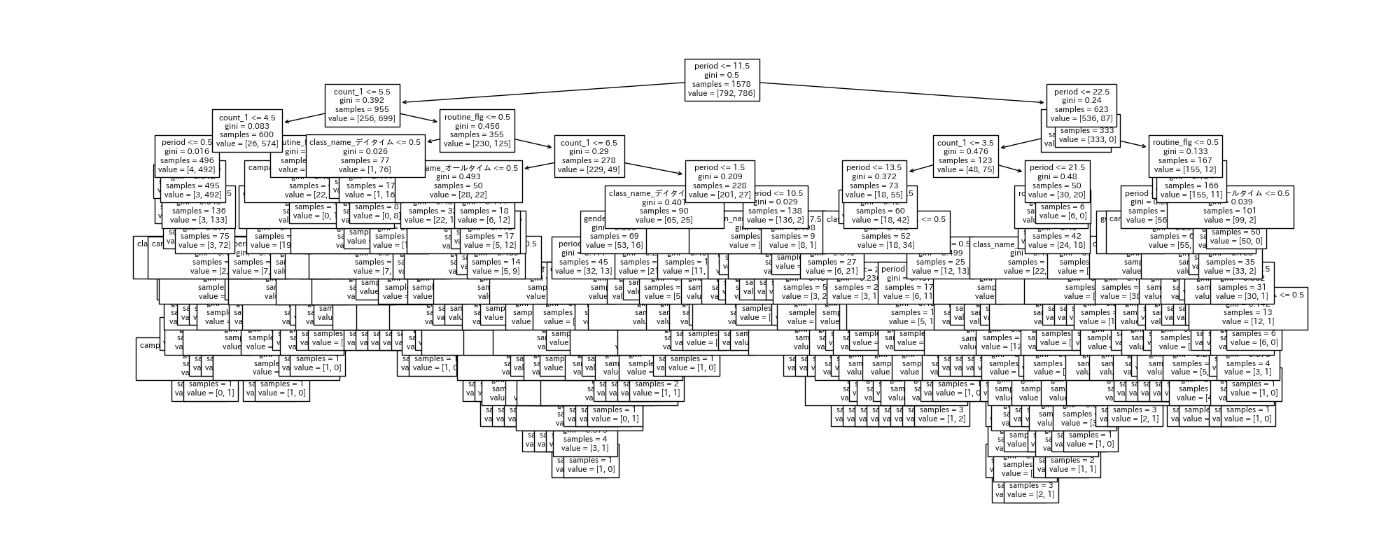
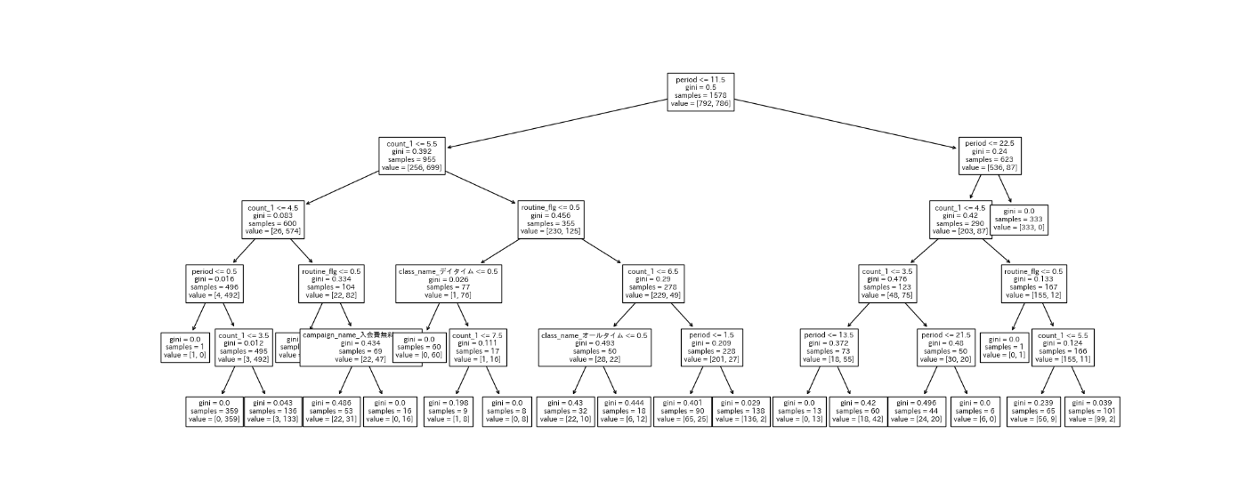
大分深くなっているため、今回はmat_depthを5と調整して、再度学習を行います。
%%time

# 本当はモデル名は区別できるようにしておいた方が良いが、今回はテキストに合わせている
model = DecisionTreeClassifier(random_state = 0,
                               max_depth    = 5    # 深さを
                              )

# チューニングを行ったうえで再度学習
model.fit(X_train, y_train)

# 結果を確認
PrintColor(f'\n model.score(X_test, y_test)')
print(model.score(X_test, y_test))

PrintColor(f'n model.score(X_trian, y_train)')
print(model.score(X_train, y_train))

print()
collect()
Knock49:モデルに寄与している変数を確認する
%%time

importance = pd.DataFrame({'feature_names' : X.columns, 'coefficient' : model.feature_importances_})

PrintColor(f'\n feature importance')
display(importance)

print()
collect()
木構造を可視化してみます。
%%time

plt.figure(figsize = (20, 8))
tree.plot_tree(model,
               feature_names = X.columns.to_list(),  # X.columnsのままではエラーになるので、リスト型に変換する
               fontsize      = 8
              )

plt.savefig('Knock49_tree_after_tuning.png')

print()
collect()
Knock50:顧客の退会を予測する
%%time

# 予測データの作成
count_1       = 3
routine_flg   = 1
period        = 10
campaign_name = '入会費無料'
class_name    = 'オールタイム'
gender        = 'M'

print()
collect()
予測データをもとにデータ加工を行い、学習モデルに入れ込む準備をします。
※この部分はテキストとしてはかなり面倒な書き方をしています。本来だと元データから学習に必要な加工処理は工程が増えるため、パイプライン等で処理をまとめて簡潔にするので、少々実用的ではない部分となってしまっています。ただ、他の知識を必要としない最もシンプルなものであるともいえるので初学者には適しているとは思います。
良ければこちらのKaggleのnotebookのデータ加工を参考にしてみてください。
もしくは、予測データをDataFrameに格納したのち、Knock46の処理をそのまま適用するのが良いと思います。
%%time

if campaign_name == '入会費半額':
    # one-hotエンコーディング後のリストの並びを想定して(不要な列削除も想定済み)[1,0]としているが、この表記だとそれがわかりづらい
    campaign_name_list = [1, 0]
elif campaign_name == '入会費無料':
    campaign_name_list = [0, 1]
elif campaign_name == '通常':
    campaign_name_list = [0, 0]

if class_name == 'オールタイム':
    class_name_list = [1, 0]
elif class_name == 'デイタイム':
    class_name_list = [0, 1]
elif class_name == 'ナイト':
    class_name_list = [0, 0]

if gender == 'F':
    gender_list = [1]
elif gender == 'M':
    gender_list = [0]

print()
collect()
%%time

# 加工したデータをまとめる.テキストではextend()を用いていたが、冗長に感じたためこちらに変更
input_data = [count_1, routine_flg, period] +\
             campaign_name_list +\
             class_name_list +\
             gender_list

input_data = pd.DataFrame(data = [input_data], columns = X.columns)

# 確認用
PrintColor(f'\n input_data')
display(input_data)

print()
collect()
%%time

PrintColor(f'\n model.predict(input_data)')
print(model.predict(input_data))

PrintColor(f'\n model.predict_proba(input_data)')
print(model.predict_proba(input_data))

print()
collect()
結果としては1(退会する)と予測しました。
しかもその確率は0(退会しない)については0%で、1(退会する)については100%だといっているので
かなりの自信のようです。
ご協力のほどよろしくお願いします。
Discussion