Neurokit アルゴリズム — 心電図　QRS/Rピーク検出

Neurokit アルゴリズム — 心電図 QRS / Rピーク検出

概要

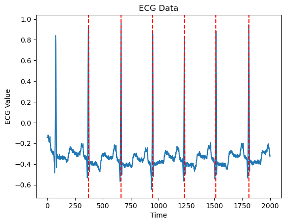
NeuroKit2は、生理信号処理のためのPythonライブラリであり、心電図（ECG）信号からRピークを検出するためのデフォルトアルゴリズムを提供している。他のアルゴリズムより、所見では精度が良いので、中身を理解するために、処理の流れを整理する。

ライブラリの結果

import neurokit2 as nk
import pandas as pd
import wfdb
import matplotlib.pyplot as plt


record = wfdb.rdrecord('100', pn_dir='mitdb')
ecg_signal = record.p_signal[:,0]

ecg_df = pd.DataFrame(ecg_signal, columns=["ecg"])


signal,info = nk.ecg_peaks(ecg_df["ecg"].values, sampling_rate=record.fs, method="neurokit")

# データの可視化
plt.plot(ecg_df["ecg"].values[:2000])  # 最初の3000サンプルをプロット
#ピークの位置に赤帽線
for peak in info["ECG_R_Peaks"]:
    if peak < 2000:  # プロット範囲内のピークのみ表示
        plt.axvline(x=peak, color='r', linestyle='--')
plt.title('ECG Data')
plt.xlabel('Time')
plt.ylabel('ECG Value')
plt.show()

アルゴリズムの流れ

NeuroKit2のRピーク検出アルゴリズムは、以下のステップで構成されている。

1. 勾配計算: ECG信号の勾配を計算し、信号の変化率を強調する。これにより、急激な変化（QRS複合体）がより明確になる。
2. 絶対値計算: 勾配の絶対値を計算し、信号の変化の大きさを強調する。これにより、正負の変化が区別されなくなる。
3. スムージング（短時間）: 短時間のスムージングを適用し、ノイズを低減する。boxcar カーネルを使用して、信号の短期的な変動を平滑化する。
4. 平均化（長時間窓）: 信号の振幅を一定の範囲にスケーリングすることで、ピーク検出の精度を向上させる。
5. 閾値計算
6. QRSの開始地点と終了地点の特定(たちあがり、たちさがり検出)
7. 不良区間の除外（短すぎるQRSのスキップ）し,各QRS内でピーク検出

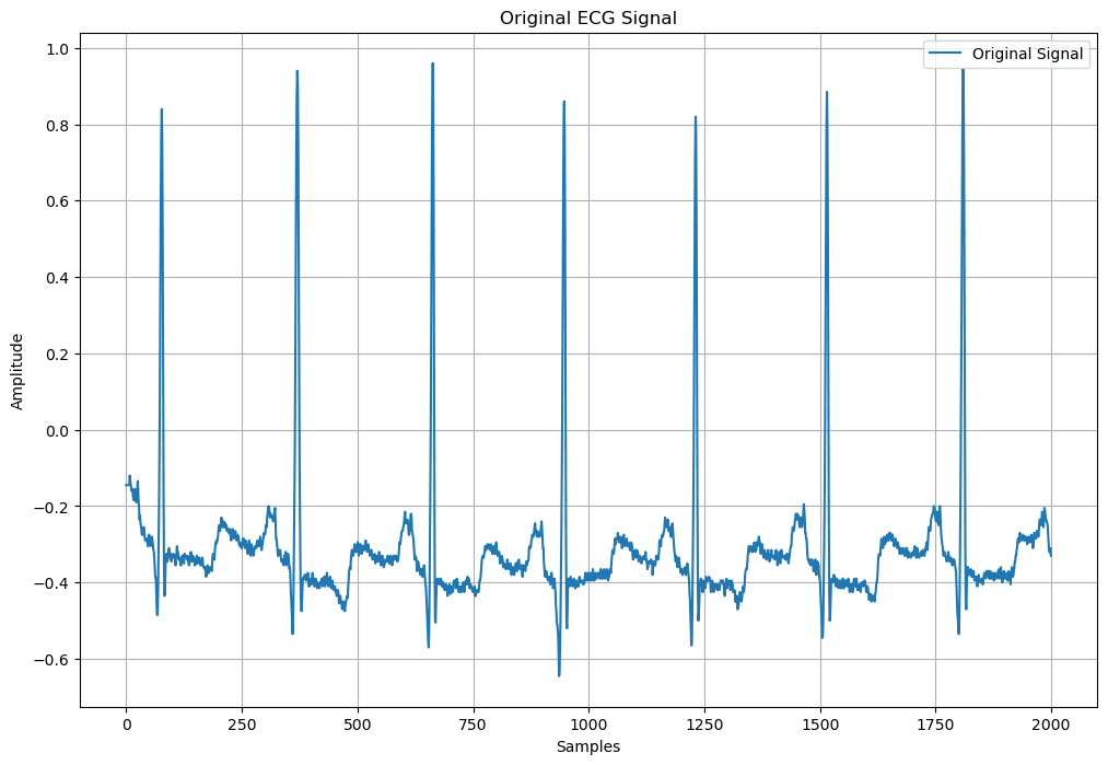
1. 勾配計算

ECG信号の勾配を計算し、信号の変化率を強調する。これにより、急激な変化（QRS複合体）がより明確になる。

import numpy as np
import matplotlib.pyplot as plt
import wfdb
from neurokit_ecg_findpeaks import signal_smooth, neurokit_findpeaks

# レコードと信号の読み込み（既に前のセルで読み込んでいれば省略可）
rec = wfdb.rdrecord('100', pn_dir='mitdb')
sig = rec.p_signal[:,0]
fs = rec.fs

plt.figure(figsize=(12, 8))
plt.plot(sig[:2000])
plt.legend(['Original Signal'])
plt.title('Original ECG Signal')
plt.xlabel('Samples')
plt.ylabel('Amplitude')
plt.grid()
plt.show()


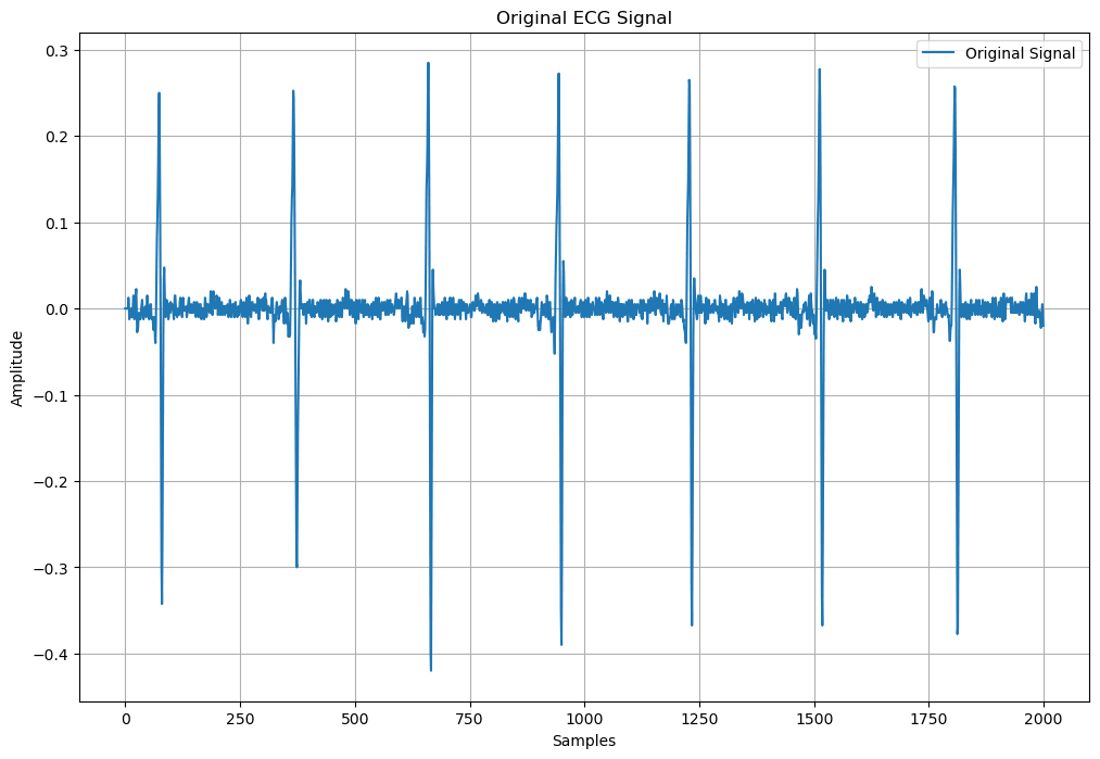
#1.勾配計算(試しに2000サンプルで計算)

grad = np.gradient(sig[:2000])


plt.figure(figsize=(12, 8))
plt.plot(grad)
plt.legend(['Original Signal'])
plt.title('Original ECG Signal')
plt.xlabel('Samples')
plt.ylabel('Amplitude')
plt.grid()
plt.show()

心電図データ	勾配計算

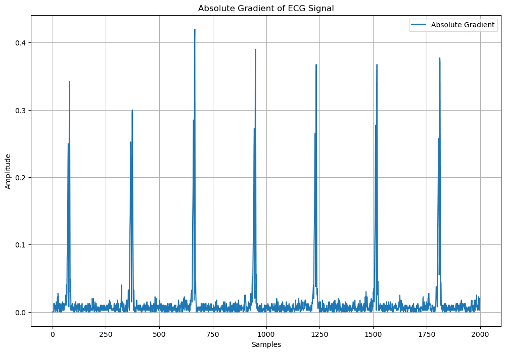
2. 絶対値計算

勾配の絶対値を計算し、信号の変化の大きさを強調する。これにより、正負の変化が区別されなくなる。

#絶対値に変換
absgrad = np.abs(grad)
plt.figure(figsize=(12, 8))
plt.plot(absgrad)
plt.legend(['Absolute Gradient'])
plt.title('Absolute Gradient of ECG Signal')
plt.xlabel('Samples')
plt.ylabel('Amplitude')
plt.grid()
plt.show()

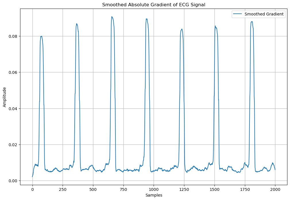
3. スムージング（短時間）

短時間のスムージングを適用し、ノイズを低減する。boxcar カーネルを使用して、信号の短期的な変動を平滑化する。

# 短時間スムージング
def signal_smooth(x, kernel='boxcar', size=3):
    if kernel != 'boxcar':
        raise ValueError('Only boxcar kernel supported in this minimal port')
    if size <= 1:
        return x
    window = np.ones(size) / size
    return np.convolve(x, window, mode='same')


smoothwindow = 0.1
smooth_kernel = int(np.rint(smoothwindow * fs))#fs上で使用した値

#平滑化
smoothgrad = signal_smooth(absgrad, kernel='boxcar', size=max(1, smooth_kernel))

#boxcar 平滑化の結果をプロット
plt.figure(figsize=(12, 8))
plt.plot(smoothgrad)
plt.legend(['Smoothed Gradient'])
plt.title('Smoothed Absolute Gradient of ECG Signal')
plt.xlabel('Samples')
plt.ylabel('Amplitude')
plt.grid()
plt.show()

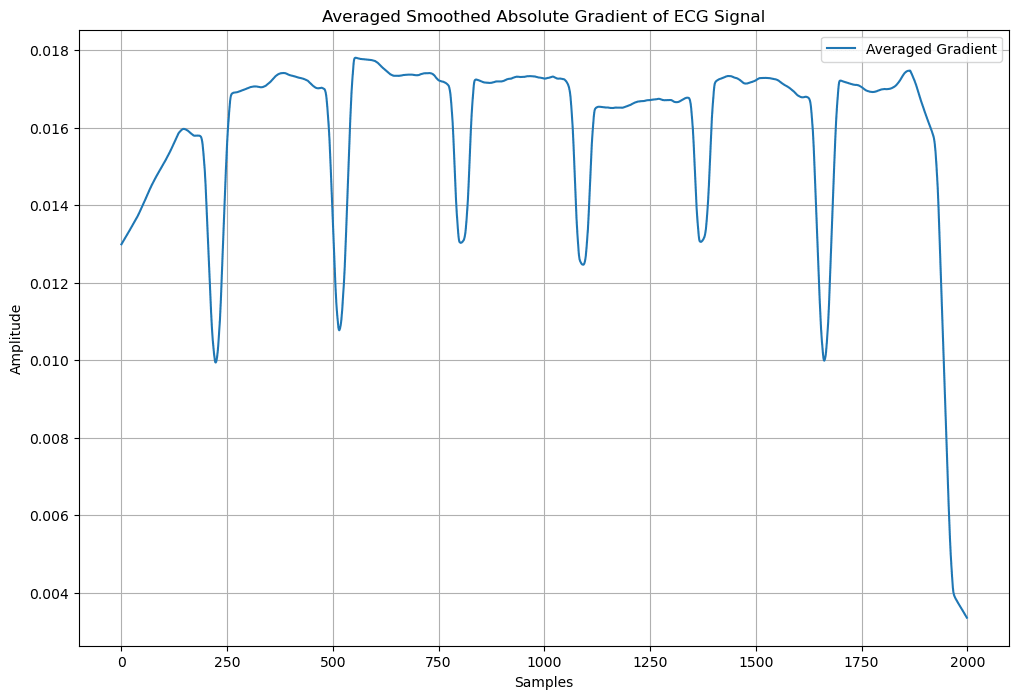
4. 平均化（長時間窓）

長時間の移動平均を適用し、信号の全体的な傾向を捉える。これにより、ピーク検出の基準となる信号が得られる。

def signal_smooth(x, kernel='boxcar', size=3):
    if kernel != 'boxcar':
        raise ValueError('Only boxcar kernel supported in this minimal port')
    if size <= 1:
        return x
    window = np.ones(size) / size
    return np.convolve(x, window, mode='same')

avgwindow=0.75

avg_kernel = int(np.rint(avgwindow * fs))
#平均化
avggrad = signal_smooth(smoothgrad, kernel='boxcar', size=max(1, avg_kernel))

plt.figure(figsize=(12, 8))
plt.plot(avggrad) 
plt.legend(['Averaged Gradient'])
plt.title('Averaged Smoothed Absolute Gradient of ECG Signal')
plt.xlabel('Samples')
plt.ylabel('Amplitude')
plt.grid()
plt.show()

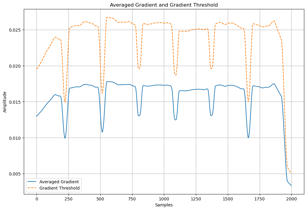
5. 閾値計算

QRSの開始地点と終了地点決定するための閾値を計算する。
平均化された信号の一定の割合を閾値として設定する。

gradthreshweight = 1.5
gradthreshold = gradthreshweight * avggrad

plt.figure(figsize=(12, 8))
plt.plot(avggrad, label='Averaged Gradient')
plt.plot(gradthreshold, label='Gradient Threshold', linestyle='--')
plt.legend()
plt.title('Averaged Gradient and Gradient Threshold')
plt.xlabel('Samples')
plt.ylabel('Amplitude')
plt.grid()
plt.show()

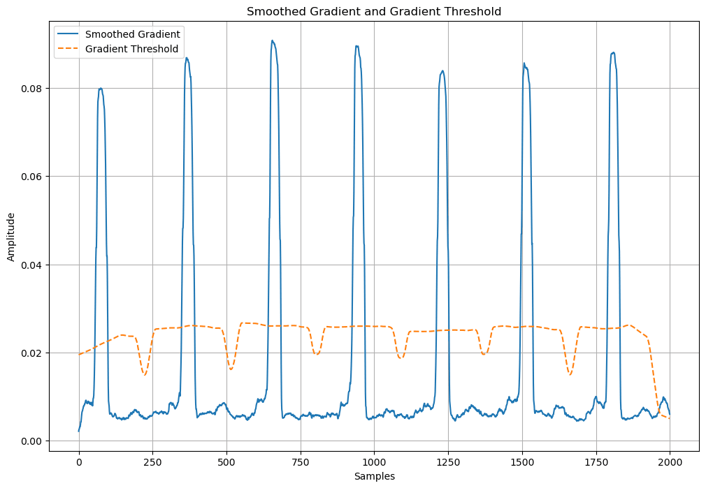
6. QRSの開始地点と終了地点の特定(たちあがり、たちさがり検出)

作成した閾値を使用して、QRS複合体の開始地点と終了地点を特定する。
これにより、各QRS複合体の範囲が明確になる

# QRSの開始地点と終了地点の特定できる閾値になる
plt.figure(figsize=(12, 8))
plt.plot(smoothgrad, label='Smoothed Gradient')
plt.plot(gradthreshold, label='Gradient Threshold', linestyle='--')
plt.legend()
plt.title('Smoothed Gradient and Gradient Threshold')
plt.xlabel('Samples')
plt.ylabel('Amplitude')
plt.grid()
plt.show()


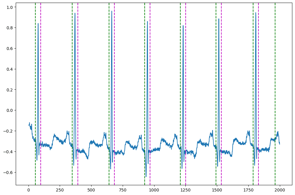
#6.立ち上がり、立ち下がり検出
qrs = smoothgrad > gradthreshold #true/falseの配列
# beg_qrs: 最初の1つの立ち上がりのインデックス
# end_qrs: 最初の1つの立ち下がりのインデックス
beg_qrs = np.where(np.logical_and(np.logical_not(qrs[0:-1]), qrs[1:]))[0]
end_qrs = np.where(np.logical_and(qrs[0:-1], np.logical_not(qrs[1:])))[0]
end_qrs = end_qrs[end_qrs > beg_qrs[0]]



#beg_qrs end_qrs 可視化
plt.figure(figsize=(12, 8))
plt.plot(sig[:2000], label='ECG Signal')
for beg in beg_qrs:
    if beg < 2000:
        plt.axvline(x=beg, color='g', linestyle='--', label='QRS Onset' if 'QRS Onset' not in plt.gca().get_legend_handles_labels()[1] else "")
for end in end_qrs:
    if end < 2000:
        plt.axvline(x=end, color='m', linestyle='--', label='QRS Offset' if 'QRS Offset' not in plt.gca().get_legend_handles_labels()[1] else "")

7. 不良区間の除外（短すぎるQRSのスキップ）し,各QRS内でピーク検出

最後に、各QRS複合体内でRピークを検出する。短すぎるQRS複合体は除外し、各QRS内で最も顕著なピークを特定する。

#分割した範囲ないでscipy.signal.find_peaksを使ってRピークを検出

import scipy.signal

minlenweight = 0.4
mindelay=0.3
# Identify R-peaks within QRS (ignore QRS that are too short).
num_qrs = min(beg_qrs.size, end_qrs.size)
mindelay = int(np.rint(fs * mindelay))
min_len = np.mean(end_qrs[:num_qrs] - beg_qrs[:num_qrs]) * minlenweight
peaks = [0]

for i in range(num_qrs):
    beg = beg_qrs[i]
    end = end_qrs[i]
    len_qrs = end - beg

    if len_qrs < min_len:
        continue

    # Find local maxima and their prominence within QRS.
    data = sig[beg:end]
    
    locmax, props = scipy.signal.find_peaks(data, prominence=(None, None))

    if locmax.size > 0:
        # Identify most prominent local maximum.
        peak = beg + locmax[np.argmax(props["prominences"])]
        #最も顕著な局所最大値を特定します。
        if peak - peaks[-1] > mindelay:
            peaks.append(peak)

peaks.pop(0)

# Rピーク検出結果を可視化
plt.figure(figsize=(12, 8))
plt.plot(sig[:2000], label='ECG Signal')
for peak in peaks:
    if peak < 2000:
        plt.axvline(x=peak, color='r', linestyle='--', label='R Peak' if 'R Peak' not in plt.gca().get_legend_handles_labels()[1] else "")
plt.legend()
plt.title('ECG Signal with Detected R Peaks')
plt.xlabel('Samples')
plt.ylabel('Amplitude')
plt.grid()
plt.show()

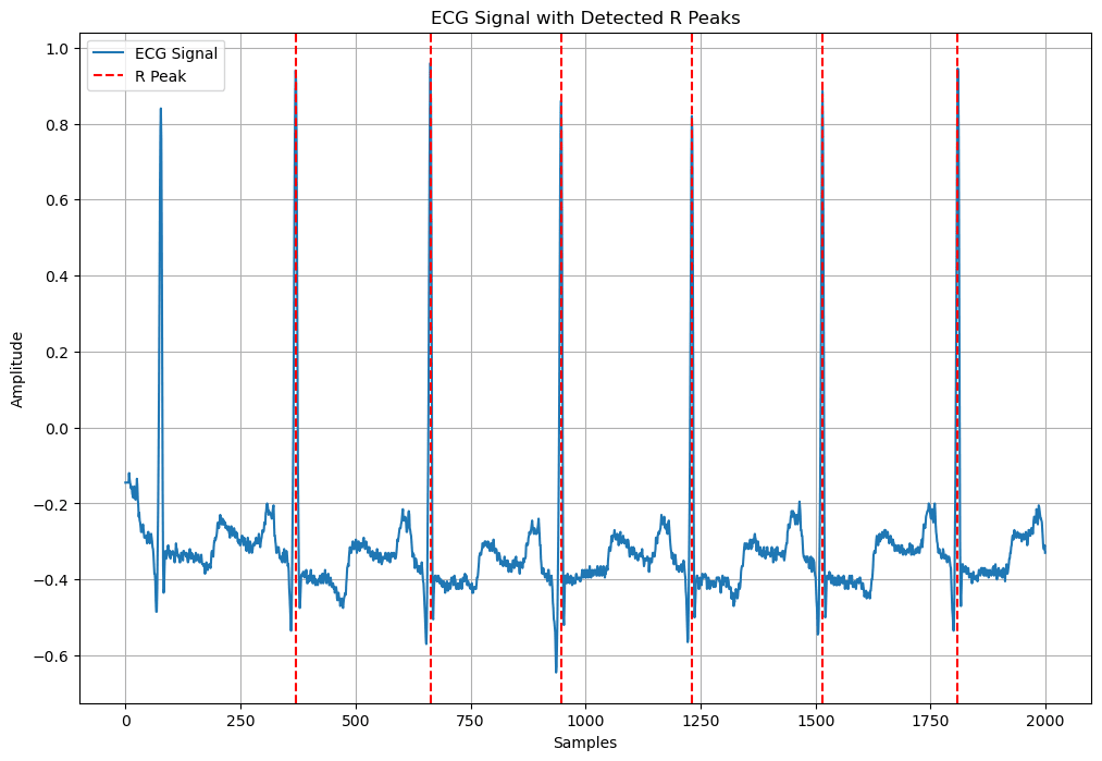
まとめ

ルールベースの検出になる。
また、結局はscipyのfind_peaksを使っているため、上に山なR波では検出できるが、マイナス側にも谷が大きくあるR波では、R波をご検出することがある。