Open15
Rで回帰分析をする上でのワークフローメモ
回帰分析で用いるコード
- 回帰分析 (交互作用項、高次分析の場合、など subset やweightの使い方は別スレッドで)
- 結果の出力
- 予測結果の出力
- 回帰診断図
- 係数の信頼区間出力
library(tidyverse)
library(gapminder)

# 1
res_lm <- lm(lifeExp ~ gdpPercap + pop + continent, data = gapminder)

# 2
summary(res_lm)

# 3. predict()

# 4.Regression diagnostic
par(mfrow = c(2, 2))
plot(res_lm) # plot(res_lm, which = c(1, 2))で出力したい診断図を指定

# 5. 係数の信頼区間の出力
coef(fit_lm)
confint(fit_lm)
2. 回帰分析の結果
summary(res_lm)
#> Call:
#> lm(formula = lifeExp ~ gdpPercap + pop + continent, data = gapminder)
#>
#> Residuals:
#>     Min      1Q  Median      3Q     Max
#> -49.161  -4.486   0.297   5.110  25.175
#>
#> Coefficients:
#>                    Estimate Std. Error t value Pr(>|t|)
#> (Intercept)       4.781e+01  3.395e-01 140.819  < 2e-16 ***
#> gdpPercap         4.495e-04  2.346e-05  19.158  < 2e-16 ***
#> pop               6.570e-09  1.975e-09   3.326 0.000901 ***
#> continentAmericas 1.348e+01  6.000e-01  22.458  < 2e-16 ***
#> continentAsia     8.193e+00  5.712e-01  14.342  < 2e-16 ***
#> continentEurope   1.747e+01  6.246e-01  27.973  < 2e-16 ***
#> continentOceania  1.808e+01  1.782e+00  10.146  < 2e-16 ***
#> ---
#> Signif. codes:  0 ‘***’ 0.001 ‘**’ 0.01 ‘*’ 0.05 ‘.’ 0.1 ‘ ’ 1
#>
#> Residual standard error: 8.365 on 1697 degrees of freedom
#> Multiple R-squared:  0.5821,	Adjusted R-squared:  0.5806
#> F-statistic: 393.9 on 6 and 1697 DF,  p-value: < 2.2e-16
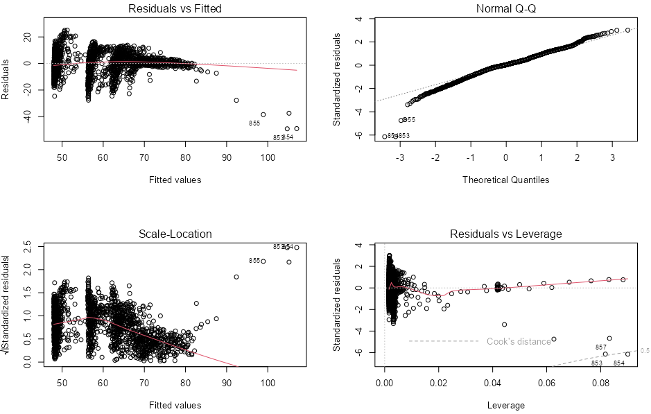
4.残差診断図
par(mfrow = c(2, 2))
plot(res_lm) # plot(res_lm, which = c(1, 2))で出力したい診断図を指定
回帰係数の信頼区間をプロットする方法
library(broom)
lm_conf <- tidy(res_lm, conf.int = TRUE)

lm_conf <- subset(lm_conf, term %nin% "(Intercept)") # socviz::%nin% > !=
lm_conf$nicelabs <- prefix_strip(lm_conf$term, "continent")

ggplot(lm_conf, aes(x = reorder(nicelabs, estimate), y = estimate, ymin = conf.low, ymax = conf.high)) +
  geom_pointrange() +
  coord_flip()

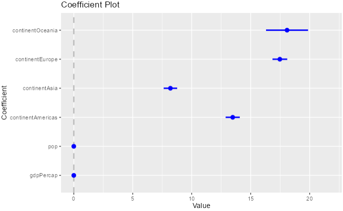
coefplot()を使う方法
library(coefplot)
coefplot(res_lm)
coefplot(res_lm, intercept = FALSE)
modelsumary()を使う方法
msummary()関数で、Viewerタブに表示される
リスト形式で与えると横に並べて比較することが可能
デフォルトでは標準誤差statistic="std.err"がデフォルトで表示されるが、
p.valueやconf.intなど出力も可能
library(modelsummary)
res_lm2 <- lm(lifeExp ~ gdpPercap + pop + continent + pop:continent, data = gapminder)

res_tab <- list()
res_tab[["Model 1"]] <- res_lm
res_tab[["Model 2"]] <- res_lm2

# - 下記のような書き方も可能
# regs <-
#  list(
#    "model1" = lm(inc ~ educ, data = saving),
#    "model2" = lm(inc ~ educ + age, data = saving)
#  )
# msummary(regs, gof_omit = 'AIC|BIC|Log.Lik.|F')

msummary(
  res_tab,
  title = "Model Comp",
  notes = list(
    "memo 1. normal term",
    "memo 2. interaction"
    ))
msummary(res_tab, statistic = "p.value")
msummary(res_tab, statistic = "conf.int", conf_level = .99) #
msummary(res_tab, gof_omit = 'AIC|BIC|Log.Lik.|F')

以下続く
参考サイト)
- gtsummaryを使った出力も今後検討
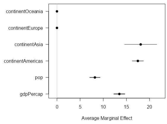
平均限界効果の出力
重回帰モデルの場合、回帰係数と平均限界効果の値は一致するが、ロジスティック回帰の場合はオッズ比である係数と平均限界効果の値は一致しない
ロジスティック回帰モデルでは限界効果は 各説明変数に依存している
library(margins)
res_marg <- margins(res_lm)
#>  gdpPercap      pop continentAmericas continentAsia continentEurope continentOceania
#>  0.0004495 6.57e-09             13.48         8.193           17.47            18.08
summary(res_marg)

par(mar = c(5, 15, 1, 1)) # bottom, left, top, right
plot(res_marg, horizontal = TRUE)
グラフの値と数値の結果が一致しないため、ggplot2()などで自分で出力したほうがいい
-
ggplot2で出力する方法
res_marg_sum <- as_tibble(summary(res_marg))

res_marg_sum <- res_marg_sum %>%
  mutate(factor = str_remove_all(factor, "continent"))

ggplot(
  res_marg_sum,
  aes(x = reorder(factor, AME), y = AME, ymin = lower, ymax = upper)
) + geom_hline(yintercept = 0, color = "gray80") +
  geom_pointrange() +
  coord_flip() +
  labs(x = NULL, y = "Average Marginal Effect")

条件付き効果の出力
library(margins)

cplot(res_lm, x = "pop")

# or ggplot out
pv_cp <- cplot(res_lm, x = "pop", draw = FALSE)

ggplot(pv_cp, aes(x = xvals, yvals, ymin = lower, ymax = upper)) +
  geom_hline(yintercept = 0, color = "gray80") +
  geom_pointrange() +
  ylim(45, 70)
-
cplot draw = TRUE
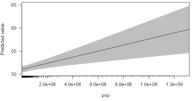
-
ggplot2

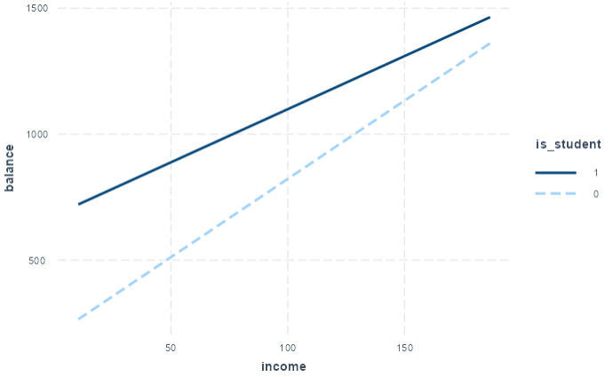
interactionsパッケージを使う方法
- pred: 交互作用項での予測変数を設定
- modx: moderator variable(調整変数)を設定
library(interactions)
credit <- Credit %>%
  mutate(
    balance = Balance,
    income = Income,
    is_student = if_else(Student == "Yes", 1, 0)
  )
lm_credit <- lm(balance ~ income * is_student, data = credit)
interact_plot(lm_credit, pred = income, modx = is_student)
参考サイト)
base Rでもプロットする方法
coef_credit <- coef(lm_credit)
plot(credit$income, credit$balance, type = "n", xlim = c(0, 200), ylim = c(0, 2000))
abline(coef_credit[1] + coef_credit[3], coef_credit[2] + coef_credit[4], col = "red")
abline(coef_credit[1], coef_credit[2], col = "black")
legend(
  "topleft",
  legend = c("is_Student=1", "is_Student=0"),
  col = c("red", "black"),
  lty = c("solid", "solid")
)

多項式回帰をするときの注意点 I() v.s. poly()
lm(mpg ~ poly(horsepower, 2), data = Auto)
lm(mpg ~ poly(horsepower, 2, raw = TRUE), data = Auto)
lm(mpg ~ horsepower + I(horsepower^2), data = Auto)

#> Call:
#> lm(formula = mpg ~ poly(horsepower, 2), data = Auto)
#>
#> Coefficients:
#>          (Intercept)  poly(horsepower, 2)1  poly(horsepower, 2)2
#>                23.45               -120.14                 44.09
#>
#>
#> Call:
#> lm(formula = mpg ~ poly(horsepower, 2, raw = TRUE), data = Auto)
#>
#> Coefficients:
#>                      (Intercept)  poly(horsepower, 2, raw = TRUE)1  poly(horsepower, 2, raw = TRUE)2
#>                        56.900100                         -0.466190                          0.001231
#>
#>
#> Call:
#> lm(formula = mpg ~ horsepower + I(horsepower^2), data = Auto)
#>
#> Coefficients:
#>     (Intercept)       horsepower  I(horsepower^2)
#>       56.900100        -0.466190         0.001231
I(x^2) = poly(x, 2, raw = TRUE)
poly()は
falseの場合はただ単に、〇乗を返してくれるだけではないようです。まずは〇乗して、スケーリングを実施して、その後直交行列を返してくれるようです。なぜ、このような計算が必要なのでしょうか?理由としては、2つ提案されています。
1 ある数字の2乗、3乗を変数にすると、それらがcorrelationを強く持ち、multicollinearityを起こしてしまう。そのため、変数たちがmulticollinearityを起こさないために直交化させる必要がある。
2 直交化しない場合には、例えば2乗の項までで回帰分析したときに得られた変数の係数と、それに3乗の項を追加して解析したときに得られる変数の係数が大きく変わってしまいます。直交化することで、係数が大きく変わることを防ぐことができるそうです。
参考サイト)