二輪車の運動特性(1) ベンチマーク自転車モデルの固有値解析
システム行列の固有値・固有ベクトルと挙動との関係がわかったので、次はいよいよ二輪車の安定性解析モデルについて固有値・固有ベクトルを求めて、どのような挙動を示すのかを見ていきたいと思います。
二輪車安定性解析モデルのシステム行列
二輪車の運動方程式は次のように表されることを紹介しました。
これも倒立振子の場合と同様の手法で二階常微分方程式の一階化を行います。質量行列
このシステム行列を
について固有値・固有ベクトルを求めれば二輪車の運動特性がわかるのですが、これを数式的に表すことは非現実的であり、通常は数値を代入して数値計算で求めることになります。
ベンチマーク自転車の固有値
ここでは、Meijaardらの論文[1]に記載されているベンチマーク自転車の諸元を使用し、Scilabによって車速
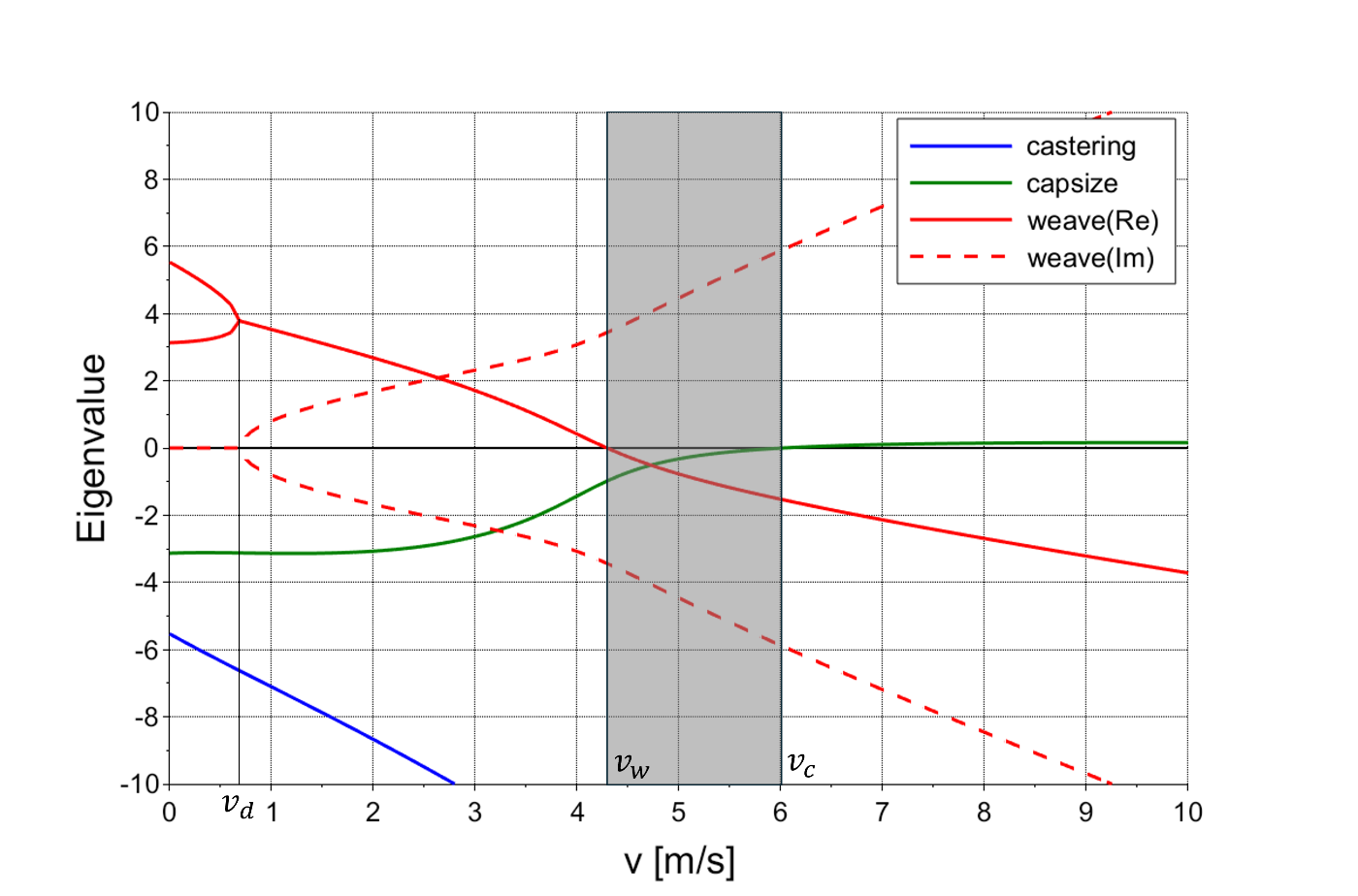
固有値の実部を実線、虚部を破線で表し、複素数のペアを同じ色で表しています。車速
グレーに塗った車速
一方、
ベンチマーク自転車の固有モード
まず、車速
sl=BicycleSys(5,9.81,M,K0,K2,C1);
[V D]=spec(sl.A);
を実行すると車速
車速
Scilabで計算された固有ベクトルは、ベクトルの大きさが1になるように正規化されていますが、固有ベクトルは方向だけを表していて大きさは不定なので、見やすくするためにここでは
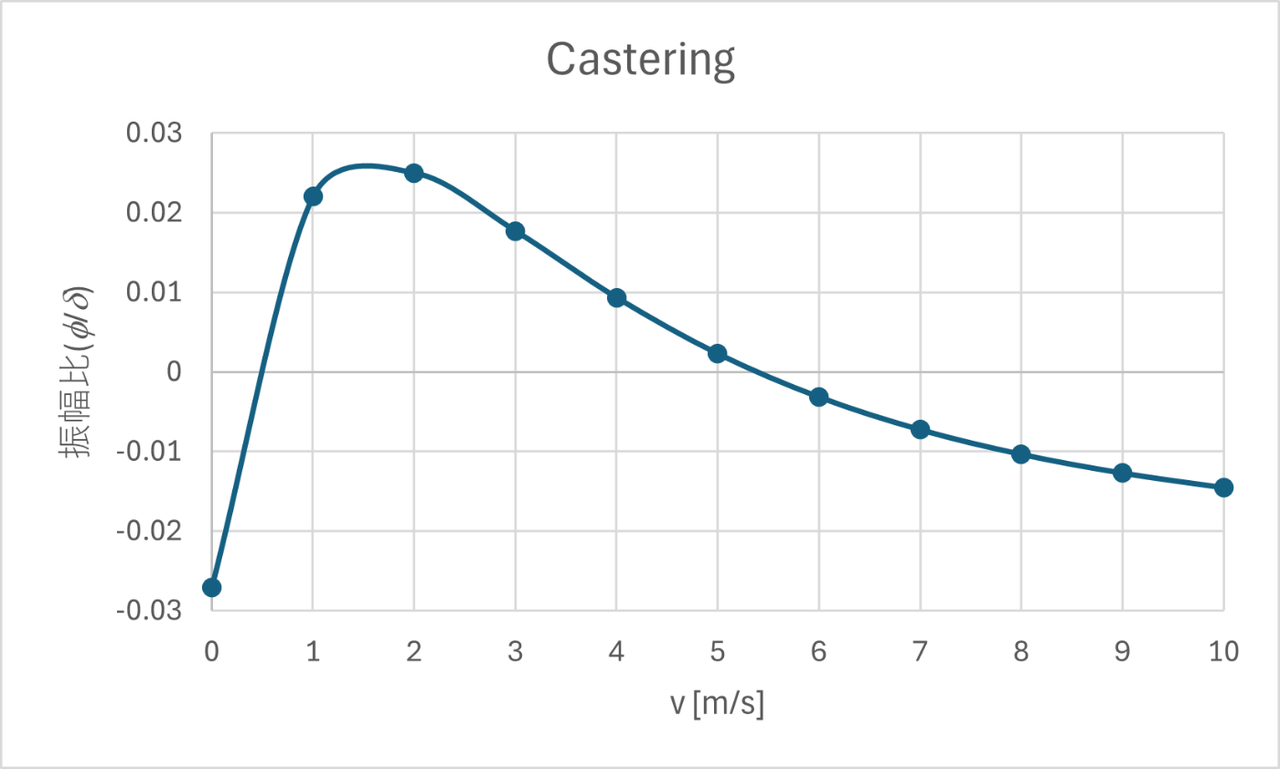
キャスタリングモード
一つ目のモードの固有値は
速度ごとに固有ベクトルの振幅比を算出すると以下のようなグラフとなり、ほぼ速度によらず常に舵角
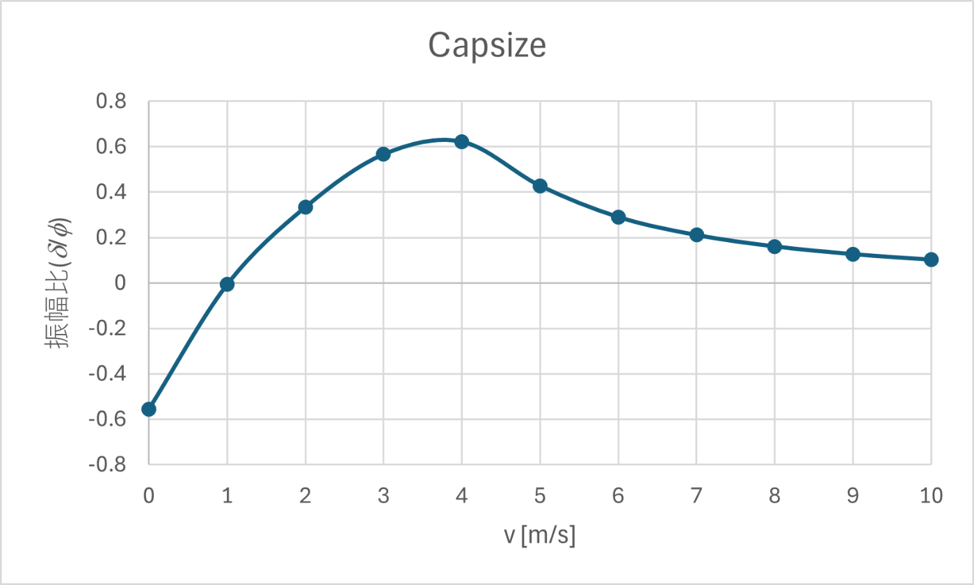
キャプサイズモード
二つ目のモードの固有値は
固有ベクトルはロール角
ウィーブモード
三つ目のモードの固有値は
複素固有値の場合、固有ベクトルも複素数となり、複素平面上での極形式表現により絶対値と偏角の情報が得られます。ここから
振幅比はおおむね0.6から0.8でロール角のほうがやや小さいですが、舵角もロール角も左右に振動するモードであり、タイヤの拘束によって舵角に比例してヨーレートが生じるため、車体全体が左右に傾きながら蛇行する挙動を示すモードです。このようにうねうねと蛇行する挙動(weave)からウィーブモードと呼ばれています。
位相をみると、ウィーブモードが安定な


車速が
まとめ
二輪車の挙動には、キャスタリング、キャプサイズ、ウィーブの3つの特徴的なモードがあり、ある程度速度が出ると自己安定性を示して倒れずに走るできることが固有値解析の結果からいえることがわかりました。また、高速ではキャプサイズモードが、低速ではウィーブモードが不安定になることが理論的に示されました。
ウィーブモードの安定・不安定の境界となる速度
//================================================
// Eigenvalue Analysis for the benchmark bicycle
//================================================
clear;
// Define Bicycle Specifications
function bicycle=DefBicycleSpec()
    bicycle.w = 1.02; // Wheel base
    bicycle.c = 0.08; // Trail
    bicycle.lambda = %pi/10; // Steer axis tilt
    bicycle.g = 9.81; // Gravity
    //// Rear WHeel R
    bicycle.rR = 0.3; // Radius
    bicycle.mR = 2; // Mass
    bicycle.IRxx = 0.0603; // Mass moment of inertia xx
    bicycle.IRyy = 0.12; // Mass moment of inertia yy
    //// Rear Body and frame assembly B
    bicycle.xB = 0.3; // Position centre of mass x
    bicycle.zB = -0.9; //Position centre of mass z
    bicycle.mB = 85; // Mass
    bicycle.IBxx = 9.2; // Mass moment of inertia xx
    bicycle.IByy = 11; // Mass moemnt of inertia yy
    bicycle.IBzz = 2.8; // Mass moement of inertia zz
    bicycle.IBxz = 2.4; // Mass product of inertia xz
    //// Front Handlebar and fork assembly H
    bicycle.xH = 0.9; // Position centre of mass x
    bicycle.zH = -0.7; // Position centre of mass z
    bicycle.mH = 4; // Mass
    bicycle.IHxx = 0.05892; // Mass moment of inertia xx
    bicycle.IHyy = 0.06; // Mass moment of inertia yy
    bicycle.IHzz = 0.00708; // Mass moment of inertia zz
    bicycle.IHxz = -0.00756; // Mass product of inertia xz
    //// Front wheel F
    bicycle.rF = 0.35; //Radius
    bicycle.mF = 3; // Mass
    bicycle.IFxx = 0.1405; // Mass moment of inertia xx
    bicycle.IFyy = 0.28; // Mass moemnt of inertia yy
endfunction
//
// Create Bicycle Matrices
function[M, K0, K2, C1]=BicycleMatrices(b)
    // Total system T properties
    mT = b.mR + b.mB + b.mH + b.mF; // Mass
    xT = (b.xB*b.mB + b.xH*b.mH + b.w*b.mF)/mT; // Position centre of mass x
    zT = (-b.rR*b.mR + b.zB*b.mB + b.zH*b.mH - b.rF*b.mF)/mT; // Position centre of mass z
    ITxx = b.IRxx + b.IBxx + b.IHxx + b.IFxx + b.mR*b.rR^2 + b.mB*b.zB^2 + b.mH*b.zH^2 + b.mF*b.rF^2;
    ITxz = b.IBxz + b.IHxz - b.mB*b.xB*b.zB - b.mH*b.xH*b.zH + b.mF*b.w*b.rF;
    ITzz = b.IRxx + b.IBzz + b.IHzz + b.IFxx + b.mB*b.xB^2 + b.mH*b.xH^2 + b.mF*b.w^2;
    // front assembly A properties
    mA = b.mH + b.mF; // Mass
    xA = (b.xH*b.mH + b.w*b.mF)/mA; // Position centre of mass x
    zA = (b.zH*b.mH - b.rF*b.mF)/mA; // Position centre of mass z
    IAxx = b.IHxx + b.IFxx + b.mH*(b.zH - zA)^2 + b.mF*(b.rF + zA)^2;
    IAxz = b.IHxz - b.mH*(b.xH - xA)*(b.zH - zA) + b.mF*(b.w - xA)*(b.rF + zA);
    IAzz = b.IHzz + b.IFxx + b.mH*(b.xH - xA)^2 + b.mF*(b.w - xA)^2;
    uA = (xA - b.w - b.c)*cos(b.lambda) - zA*sin(b.lambda);
    IAll = mA*uA^2 + IAxx*sin(b.lambda)^2 + 2*IAxz*sin(b.lambda)*cos(b.lambda) + IAzz*cos(b.lambda)^2;
     IAlx = -mA*uA*zA + IAxx*sin(b.lambda) + IAxz*cos(b.lambda);
     IAlz = mA*uA*xA + IAxz*sin(b.lambda) + IAzz*cos(b.lambda);
     // Other parameters
     mu = (b.c/b.w)*cos(b.lambda);
     SR = b.IRyy/b.rR;
     SF = b.IFyy/b.rF;
     ST = SR + SF;
     SA = mA*uA + mu*mT*xT;
     // Coefficient Matrices
     M = [ITxx IAlx+mu*ITxz; IAlx+mu*ITxz IAll+2*mu*IAlz+mu^2*ITzz];
     K0 = [mT*zT -SA; -SA -SA*sin(b.lambda)];
     K2 = [0 (ST-mT*zT)*cos(b.lambda)/b.w; 0 (SA+SF*sin(b.lambda))*cos(b.lambda)/b.w];
     C1 = [0 mu*ST+SF*cos(b.lambda)+ITxz*cos(b.lambda)/b.w-mu*mT*zT; -(mu*ST+SF*cos(b.lambda)) IAlz*cos(b.lambda)/b.w+mu*(SA+ITzz*cos(b.lambda)/b.w)];
endfunction
//
// Create Bicycle System
function sl=BicycleSys(v,g,M,K0,K2,C1)
    MI = inv(M);
    gMIK0 = g*MI*K0;
    MIK2 = MI*K2;
    MIC1 = MI*C1;
    A = [zeros(2,2) eye(2,2); -(gMIK0 + v^2*MIK2) -v*MIC1];
    B = [zeros(2,2); MI];
    C = [eye(2,2) zeros(2,2)];
    D = zeros(2,2);
    sl = syslin('c', A,B,C,D);
endfunction
//
// Main routine
// Eigenvalue Calculation
bicycle = DefBicycleSpec();
[M K0 K2 C1]=BicycleMatrices(bicycle);
v=[0:0.1:0.68428307889246,0.7:0.1:10];
i=0;
for vi=v
    i=i+1;
    sl=BicycleSys(vi,bicycle.g,M,K0,K2,C1);
    [V D]=spec(sl.A);
    D=diag(D).';
    sort_key=[abs(imag(D)); real(D)];
    [dmy idx]=gsort(sort_key,"lc","i");
    E(i,:)=D(idx);
end
//
// Draw Eigenvalue Plots
f=scf();
f.axes_size=[600 600];
// add origin axis
xpoly([v(1),v($)],[0,0],'lines');
e = gce();
e.thickness = 2;
e.line_style = 1;
e.foreground = color("black");
// plot eigenvalues
plot(v,[E(:,1),E(:,2),real(E(:,3)),imag(E(:,3))]);
xlabel("v [m/s]"),xgrid(),ylabel("Eigenvalue");
// adjust the imaginary line style and the color to the real one
h1 = gce().children;
h1(1).foreground=h1(2).foreground;
h1(1).line_style=3;
// add the plot for the conjugate complex data
plot(v,[real(E(:,4)),imag(E(:,4))]);
h2 = gce().children;
h2(1).line_style=3;
h2.foreground=h1(2).foreground;
// ajust the y scale
replot([0 -10 10 10]);
// add legend
l=legend(h1(4:-1:1),['castering','capsize','weave(Re)','weave(Im)']);
-
J. P. Meijaard, et al., "Linearized dynamics equations for the balance and steer of a bicycle: a benchmark and review", Proc. R. Soc. A 463:1955-1982, 2007 ↩︎
Discussion