PyMC 入門

PyMC 入門

PyMC は Python でベイズ統計モデリングを行うためのライブラリです。PyMC は、マルコフ連鎖モンテカルロ (MCMC) サンプリングや変分推論などのベイズ統計モデリングのための様々な手法を提供します。

統計モデルが簡単な場合、例えば正規分布を仮定して平均値を推定するとか、であれば厳密解を与える公式を陽に書き下すことができますが、モデルが複雑になるとそのような公式一発で解くことはできなくなります。
数値解法を用いる場合でも、例えば時系列予測とかで線型モデルを仮定すればカルマンフィルタなどの公式が利用できますが、それ以上に複雑なモデルとなると、MCMC などの方法に頼らざるを得ません。

ベイズ統計モデリングを行うための確率的プログラミング言語として有名なものに Stan があります。Stan は R や Python から利用可能です。
対して PyMC は Python の文法の枠内で統計モデリングができるライブラリです。PyMC の最新バージョンはこの記事を書いた時点では 5.16.1 になります。

インストール

pip コマンド一発でインストール出来ました。(pymc-5.16.1 と arviz-0.18.0 その他色々が導入された。）

$ pip3 install pymc ipywidgets

高速化に役立つかもしれないのでこれもインストールしておきます。

$ pip3 install numpyro blackjax nutpie

簡単な例：線型回帰

PyMC のチュートリアル "A Motivating Example: Linear Regressio" を元に動かしてみます。

以下、notebook で作業します。

$ jupyter notebook

色々 import して準備します。

import arviz as az
import pandas as pd
import matplotlib.pyplot as plt
import numpy as np

%config InlineBackend.figure_format = 'retina'
# Initialize random number generator
RANDOM_SEED = 8927
rng = np.random.default_rng(RANDOM_SEED)
az.style.use("arviz-darkgrid")

今回解きたいモデルは下記のような線型モデルです。

$$Y_{\text{true}} = \alpha + \beta_0 X_0 + \beta_1 X_1$$

$$Y \sim \mathcal{N}(Y_{\text{true}}, \sigma^2)$$

解くべきデータを生成します。

# 推定したい真のパラメータ
alpha, sigma = 1, 1
beta = [1, 2.5]

# データセットの大きさ
size = 100

# 確率変数 X0, X1
X0 = np.random.randn(size)
X1 = np.random.randn(size) * 0.2

# 観測された値
Y = alpha + beta[0] * X0 + beta[1] * X1 + rng.normal(size=size) * sigma

fig, axes = plt.subplots(1, 2, sharex=True, figsize=(10, 4))
axes[0].scatter(X0, Y, alpha=0.6)
axes[1].scatter(X1, Y, alpha=0.6)
axes[0].set_ylabel("Y")
axes[0].set_xlabel("X0")
axes[1].set_xlabel("X1");

PyMC モデルの作成

import pymc as pm

print(f"Running on PyMC v{pm.__version__}")

推定対象のパラメタ $\alpha, \beta, \sigma$ に対して次の事前分布を仮定します。

$$\alpha \sim \mathcal{N}(0, 10^2)$$

$$\beta_0, \beta_1 \sim \mathcal{N}(0, 10^2)$$

$$\sigma \sim |\mathcal{N}(0, 1^2)|$$

モデルを定義します。

basic_model = pm.Model()

with basic_model:
    # 未知パラメタに対する事前分布
    alpha = pm.Normal("alpha", mu=0, sigma=10)
    beta = pm.Normal("beta", mu=0, sigma=10, shape=2)
    sigma = pm.HalfNormal("sigma", sigma=1)

    # Y_true の式
    mu = alpha + beta[0] * X0 + beta[1] * X1

    # 観測される Y の値
    Y_obs = pm.Normal("Y_obs", mu=mu, sigma=sigma, observed=Y)

モデルを動かしてみます。

%time
with basic_model:
    # 1000 回、事後分布を抽出
    idata = pm.sample()

これぐらい簡単なモデルだと一瞬。

CPU times: user 3 µs, sys: 1e+03 ns, total: 4 µs
Wall time: 5.96 µs
Auto-assigning NUTS sampler...
Initializing NUTS using jitter+adapt_diag...
Multiprocess sampling (4 chains in 4 jobs)
NUTS: [alpha, beta, sigma]
Sampling 4 chains, 0 divergences ━━━━━━━━━━━━━━━━━━━━━━━━━━━━━━━━━━━━━━━━ 100% 0:00:00 / 0:00:00
Sampling 4 chains for 1_000 tune and 1_000 draw iterations (4_000 + 4_000 draws total) took 1 seconds.

実行のサマリはこれで表示される。

idata

パラメータ推定の様子は下記のように az.plot_trace で確認できる。

az.plot_trace(idata, combined=True);

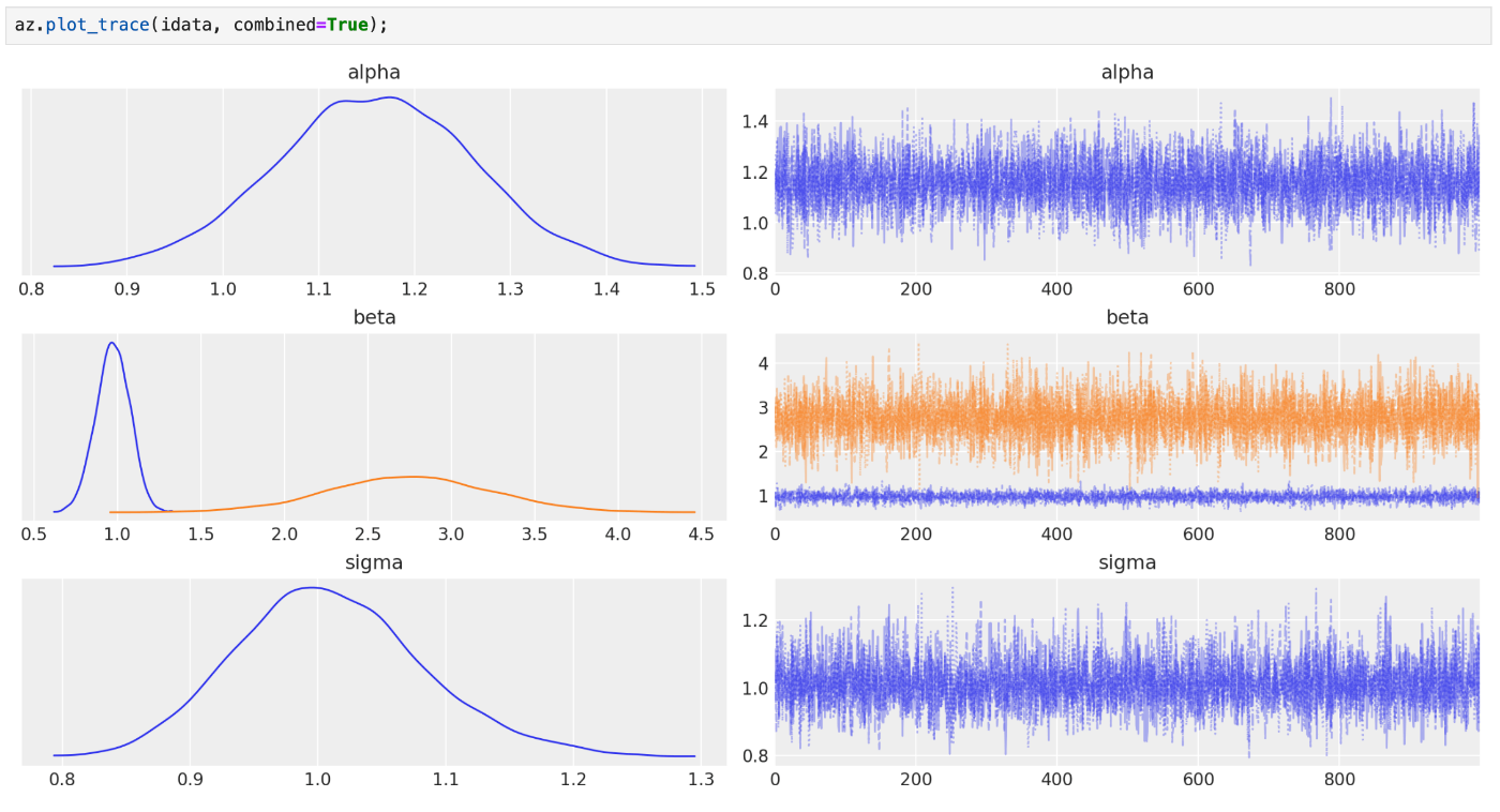
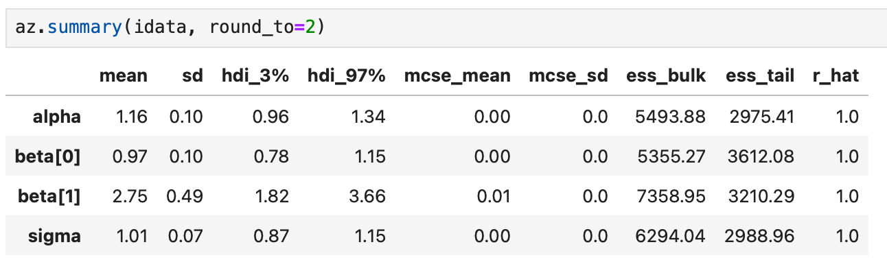
MCMCによるパラメータ推定結果は下記のように報告される。

az.summary(idata, round_to=2)

複雑な例：Coal mining disasters

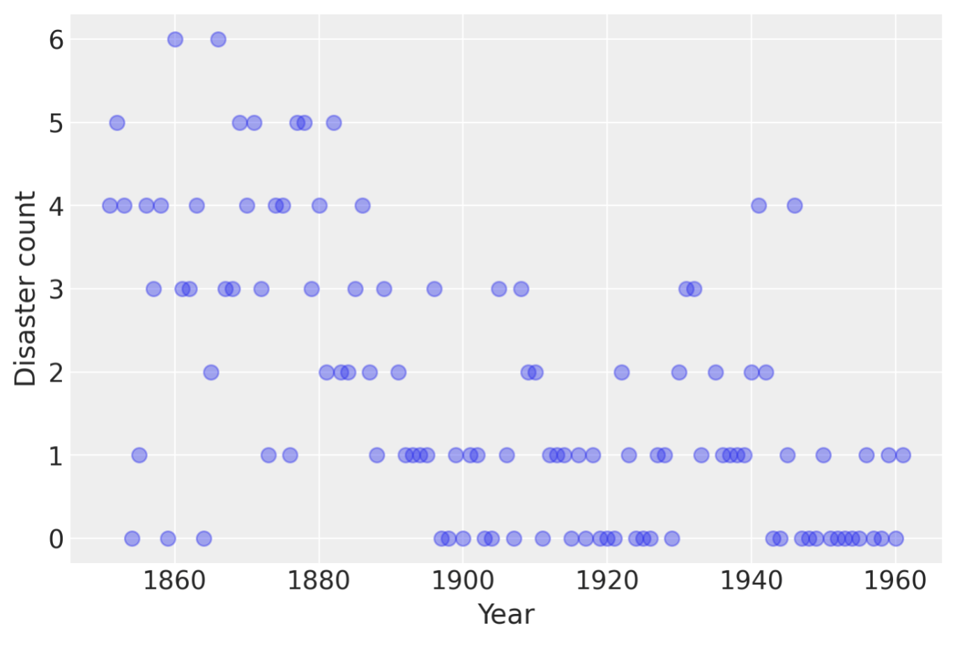
もう少し複雑な例として Case study 2: Coal mining disaster を試してみます。

これは英国での石炭鉱山での事故についてのモデルです。

# fmt: off
disaster_data = pd.Series(
    [4, 5, 4, 0, 1, 4, 3, 4, 0, 6, 3, 3, 4, 0, 2, 6,
    3, 3, 5, 4, 5, 3, 1, 4, 4, 1, 5, 5, 3, 4, 2, 5,
    2, 2, 3, 4, 2, 1, 3, np.nan, 2, 1, 1, 1, 1, 3, 0, 0,
    1, 0, 1, 1, 0, 0, 3, 1, 0, 3, 2, 2, 0, 1, 1, 1,
    0, 1, 0, 1, 0, 0, 0, 2, 1, 0, 0, 0, 1, 1, 0, 2,
    3, 3, 1, np.nan, 2, 1, 1, 1, 1, 2, 4, 2, 0, 0, 1, 4,
    0, 0, 0, 1, 0, 0, 0, 0, 0, 1, 0, 0, 1, 0, 1]
)
# fmt: on
years = np.arange(1851, 1962)

plt.plot(years, disaster_data, "o", markersize=8, alpha=0.4)
plt.ylabel("Disaster count")
plt.xlabel("Year");

各年の事故の数が与えられています。ただしデータの無い年は　np.nan で与えられています。

これを下記のようにモデル化します。

$$D_t \sim \text{Poisson}(r_t), \;\; r_t = \begin{cases}e, & \text{if } t\leq s\\l, & \text{if } t>s\end{cases},$$

$$s \sim \text{Uniform}(t_l, t_h),$$

$$e, l \sim \exp(1).$$

各年の事故数　$D_t$ はポアソン分布に従うが、その期待値 $r_t$ は、変化点 $s$ を境に $e$ から $l$ に変化する。$s$ はデータ区間で一様に分布すると考え、$e, l$は指数分布に従う。

with pm.Model() as disaster_model:
    switchpoint = pm.DiscreteUniform("switchpoint", lower=years.min(), upper=years.max())

    # Priors for pre- and post-switch rates number of disasters
    early_rate = pm.Exponential("early_rate", 1.0)
    late_rate = pm.Exponential("late_rate", 1.0)

    # Allocate appropriate Poisson rates to years before and after current
    rate = pm.math.switch(switchpoint >= years, early_rate, late_rate)

    disasters = pm.Poisson("disasters", rate, observed=disaster_data)

実行してみます。

%time
with disaster_model:
    idata = pm.sample(10000)

Multiprocess sampling (4 chains in 4 jobs)
CompoundStep
>CompoundStep
>>Metropolis: [switchpoint]
>>Metropolis: [disasters_unobserved]
>NUTS: [early_rate, late_rate]
Sampling 4 chains, 0 divergences ━━━━━━━━━━━━━━━━━━━━━━━━━━━━━━━━━━━━━━━━ 100% 0:00:00 / 0:00:04
Sampling 4 chains for 1_000 tune and 10_000 draw iterations (4_000 + 40_000 draws total) took 5 seconds.

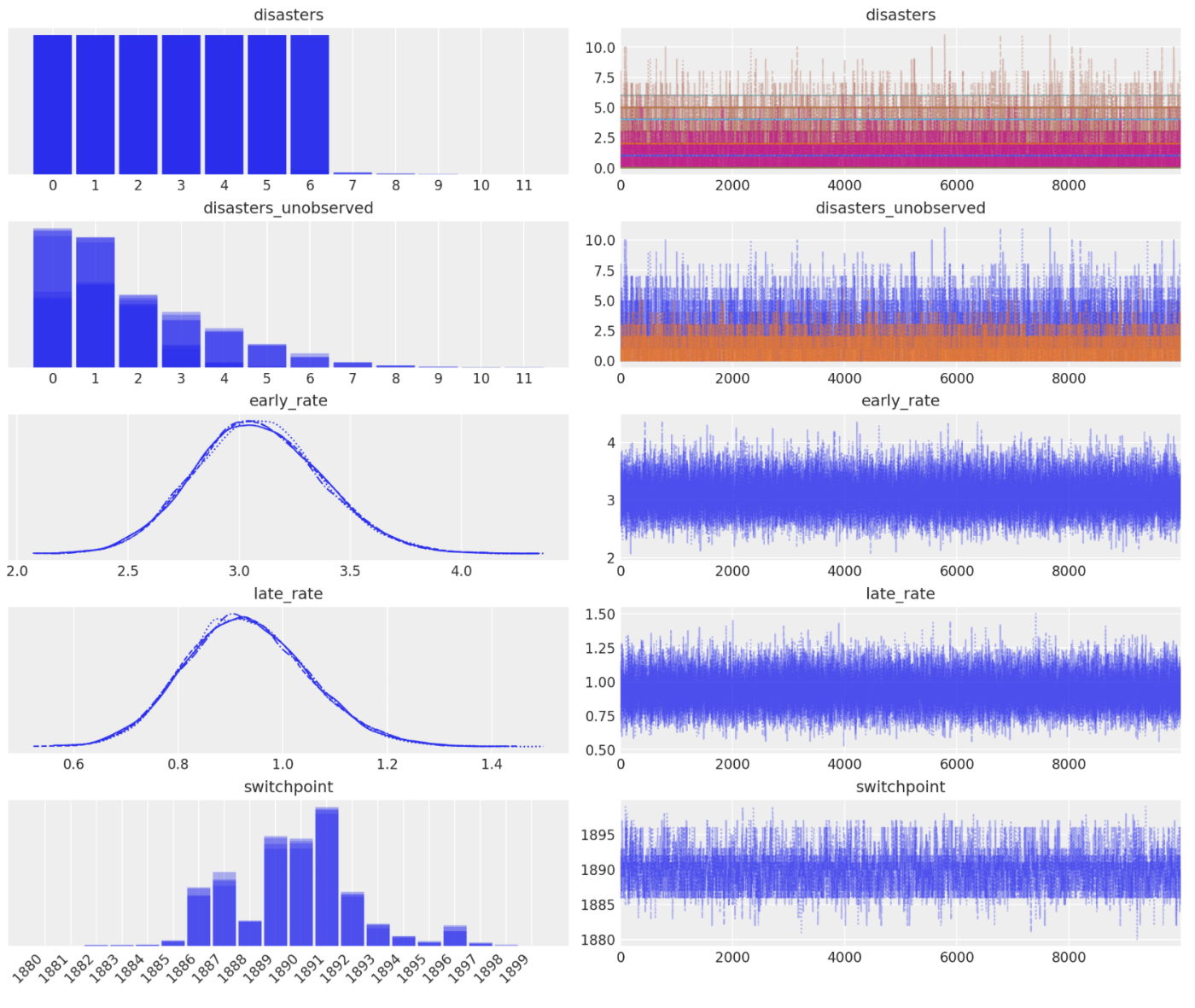
結果をグラフ表示します。（なんか switchpoint の表示に技が使われてる。）

axes_arr = az.plot_trace(idata)
plt.draw()
for ax in axes_arr.flatten():
    if ax.get_title() == "switchpoint":
        labels = [label.get_text() for label in ax.get_xticklabels()]
        ax.set_xticklabels(labels, rotation=45, ha="right")
        break
plt.draw()

plt.figure(figsize=(10, 8))
plt.plot(years, disaster_data, ".", alpha=0.6)
plt.ylabel("Number of accidents", fontsize=16)
plt.xlabel("Year", fontsize=16)

trace = idata.posterior.stack(draws=("chain", "draw"))

plt.vlines(trace["switchpoint"].mean(), disaster_data.min(), disaster_data.max(), color="C1")
average_disasters = np.zeros_like(disaster_data, dtype="float")
for i, year in enumerate(years):
    idx = year < trace["switchpoint"]
    average_disasters[i] = np.mean(np.where(idx, trace["early_rate"], trace["late_rate"]))

sp_hpd = az.hdi(idata, var_names=["switchpoint"])["switchpoint"].values
plt.fill_betweenx(
    y=[disaster_data.min(), disaster_data.max()],
    x1=sp_hpd[0],
    x2=sp_hpd[1],
    alpha=0.5,
    color="C1",
)
plt.plot(years, average_disasters, "k--", lw=2);

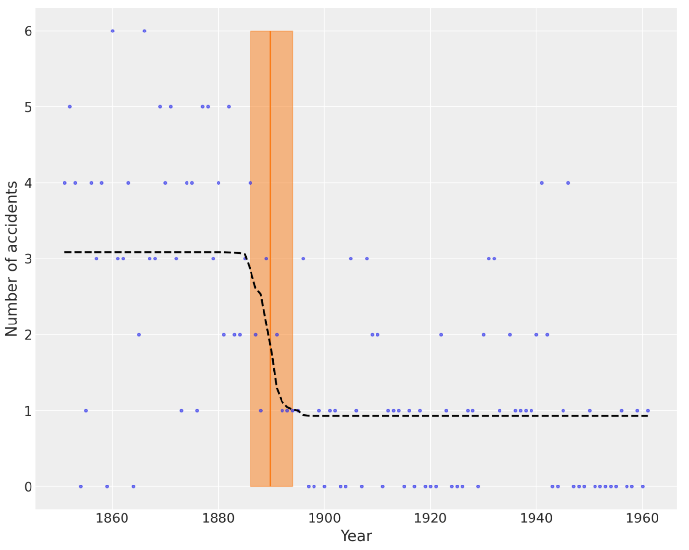
変化点検出とかは、実際の業務でもそのまま役に立ちそうなサンプルコードですね。