PyTorch で機械学習に入門する
このスクラップについて
プログラミング未経験の友達が Python の勉強を始めることに刺激を受けて僕も Python の勉強を始めてみようと思う。
最近は機械学習/ディープラーニングの凄さをまざまざと見せつけられる機会が多いので PyTorch を使って機械学習で何か面白いことをやってみようと思う。
なぜ PyTorch?
過去に TensorFlow / Keras でサンプルを動かしたけど「さて、この後はどうしようか」となったまま時が止まっている。
Getting Started
インストール
pip3 install torch torchvision torchaudio
Successfully installed MarkupSafe-2.1.2 charset-normalizer-3.1.0 filelock-3.12.0 idna-3.4 jinja2-3.1.2 mpmath-1.3.0 networkx-3.1 pillow-9.5.0 requests-2.30.0 sympy-1.12 torch-2.0.1 torchaudio-2.0.2 torchvision-0.15.2 typing-extensions-4.5.0 urllib3-2.0.2
ワークスペース作成
mkdir -p ~/workspace/python/hello-pytorch
cd ~/workspace/python/hello-pytorch
touch verification.py
コーディング
import torch
x = torch.rand(5, 3)
print(x)
実行
python3 verification.py
tensor([[0.3046, 0.3335, 0.8956],
        [0.7345, 0.9589, 0.1866],
        [0.8709, 0.7779, 0.4212],
        [0.2471, 0.7042, 0.7468],
        [0.4275, 0.0480, 0.4232]])
VSCode
まずは Python extension をインストールしたが import torch がエラーとなる。
Import "torch" could not be resolved
わかったぞ
VSCode のウィンドウの下の方にある Python をクリックするとインタープリタの一覧が表示される。
~/.pyenv/versions/3.8.2/bin/python が利用されているようだ。
それに対してターミナルで which python3 で調べると /usr/local/bin/python3 を使おうとしている。
pyenv 設定
echo 'export PYENV_ROOT="$HOME/.pyenv"' >> ~/.zshrc
echo 'command -v pyenv >/dev/null || export PATH="$PYENV_ROOT/bin:$PATH"' >> ~/.zshrc
echo 'eval "$(pyenv init -)"' >> ~/.zshrc
設定確認
which python
which pip3
/Users/susukida/.pyenv/shims/python
/Users/susukida/.pyenv/shims/pip3
もう 1 回インストール
pip3 install torch torchvision torchaudio
pip3 バージョンアップ
pip3 install --upgrade pip
VSCode で pyenv の Python を選ぶ
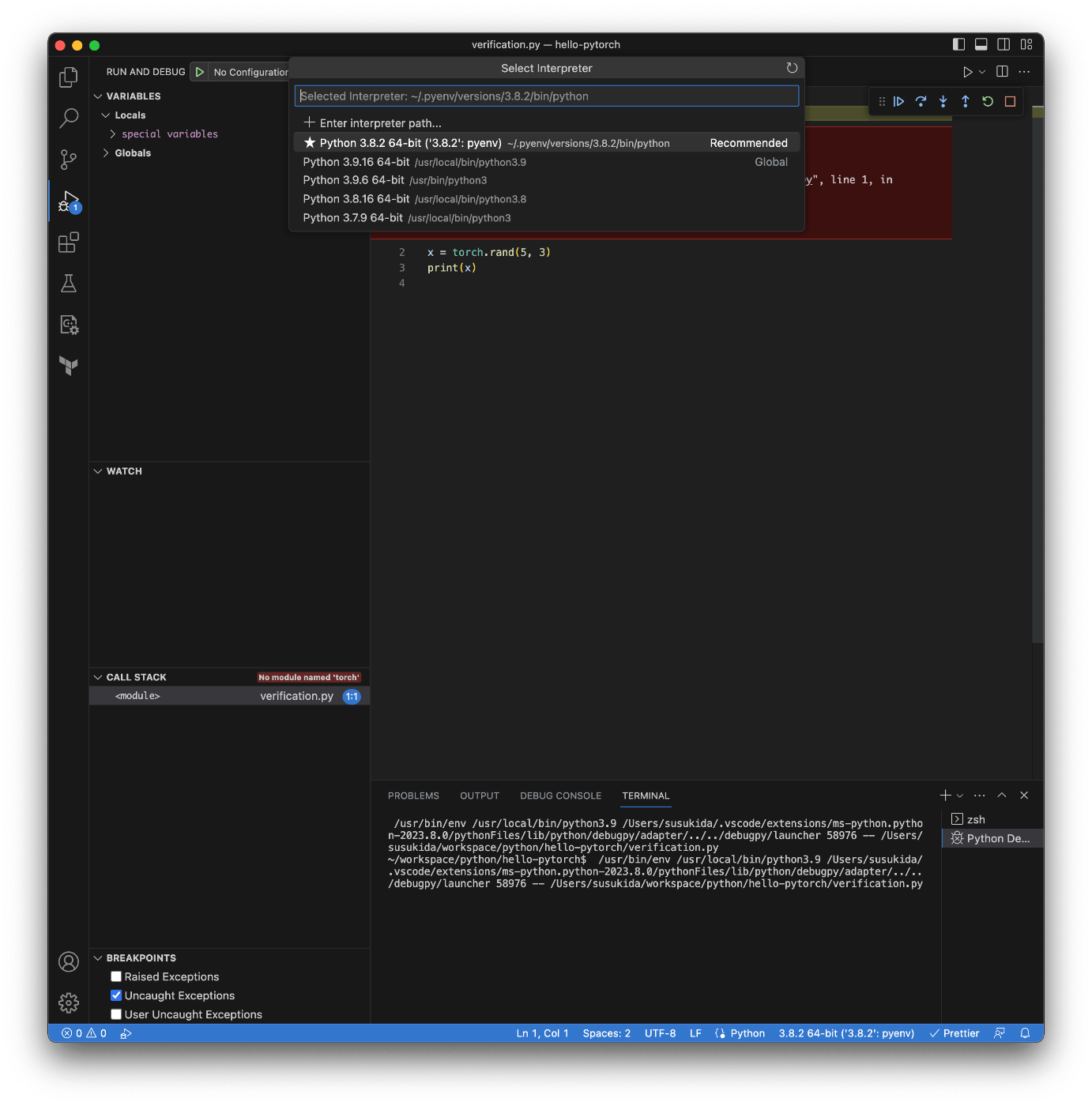
コード補完も効くし F5 実行もできる
これで準備が整った。
今日はここまで
次はクイックスタートから始めよう。
明日まで待ちきれない
touch quickstart.py
コーディング
import torch
from torch import nn
from torch.utils.data import DataLoader
from torchvision import datasets
from torchvision.transforms import ToTensor

training_data = datasets.FashionMNIST(
    root='data',
    train=True,
    download=True,
    transform=ToTensor(),
)

test_data = datasets.FashionMNIST(
    root='data',
    train=False,
    download=True,
    transform=ToTensor(),
)

batch_size = 64

train_dataloader = DataLoader(training_data, batch_size=batch_size)
test_dataloader = DataLoader(test_data, batch_size=batch_size)

device = (
    "cuda" if torch.cuda.is_available()
    else "mps" if torch.backends.mps.is_available()
    else "cpu"
)

print(device)
mps
モデル作成
import torch
from torch import nn
from torch.utils.data import DataLoader
from torchvision import datasets
from torchvision.transforms import ToTensor

training_data = datasets.FashionMNIST(
    root='data',
    train=True,
    download=True,
    transform=ToTensor(),
)

test_data = datasets.FashionMNIST(
    root='data',
    train=False,
    download=True,
    transform=ToTensor(),
)

batch_size = 64

train_dataloader = DataLoader(training_data, batch_size=batch_size)
test_dataloader = DataLoader(test_data, batch_size=batch_size)

device = (
    "cuda" if torch.cuda.is_available()
    else "mps" if torch.backends.mps.is_available()
    else "cpu"
)

print(f"Using {device} device")


class NeuralNetwork(nn.Module):
    def __init__(self):
        super().__init__()
        self.flatten = nn.Flatten()
        self.linear_relu_stack = nn.Sequential(
            nn.Linear(28*28, 512),
            nn.ReLU(),
            nn.Linear(512, 512),
            nn.ReLU(),
            nn.Linear(512, 10)
        )

    def forward(self, x):
        x = self.flatten(x)
        logits = self.linear_relu_stack(x)
        return logits


model = NeuralNetwork().to(device)
print(model)
Using mps device
NeuralNetwork(
  (flatten): Flatten(start_dim=1, end_dim=-1)
  (linear_relu_stack): Sequential(
    (0): Linear(in_features=784, out_features=512, bias=True)
    (1): ReLU()
    (2): Linear(in_features=512, out_features=512, bias=True)
    (3): ReLU()
    (4): Linear(in_features=512, out_features=10, bias=True)
  )
)
学習
mps だと pred.argmax(1) が全て 0 になるので cpu にした。
import torch
from torch import nn
from torch.utils.data import DataLoader
from torchvision import datasets
from torchvision.transforms import ToTensor

training_data = datasets.FashionMNIST(
    root='data',
    train=True,
    download=True,
    transform=ToTensor(),
)

test_data = datasets.FashionMNIST(
    root='data',
    train=False,
    download=True,
    transform=ToTensor(),
)

batch_size = 64

train_dataloader = DataLoader(training_data, batch_size=batch_size)
test_dataloader = DataLoader(test_data, batch_size=batch_size)

device = (
    "cuda" if torch.cuda.is_available()
    else "mps" if torch.backends.mps.is_available()
    else "cpu"
)
device = "cpu"


class NeuralNetwork(nn.Module):
    def __init__(self):
        super().__init__()
        self.flatten = nn.Flatten()
        self.linear_relu_stack = nn.Sequential(
            nn.Linear(28*28, 512),
            nn.ReLU(),
            nn.Linear(512, 512),
            nn.ReLU(),
            nn.Linear(512, 10)
        )

    def forward(self, x):
        x = self.flatten(x)
        logits = self.linear_relu_stack(x)
        return logits


model = NeuralNetwork().to(device)
loss_fn = nn.CrossEntropyLoss()
optimizer = torch.optim.SGD(model.parameters(), lr=1e-3)


def train(dataloader: DataLoader,
          model: NeuralNetwork,
          loss_fn: nn.CrossEntropyLoss,
          optimizer: torch.optim.SGD):
    size = len(dataloader.dataset)
    model.train()
    for batch, (X, y) in enumerate(dataloader):
        X, y = X.to(device), y.to(device)

        pred = model(X)
        loss = loss_fn(pred, y)

        loss.backward()
        optimizer.step()
        optimizer.zero_grad()

        if batch % 100 == 0:
            loss, current = loss.item(), (batch + 1) * len(X)
            print(f"loss: {loss:>7f} [{current:>5d}/{size:>5d}]")


def test(dataloader: DataLoader,
         model: NeuralNetwork,
         loss_fn: nn.CrossEntropyLoss):
    size = len(dataloader.dataset)
    num_batches = len(dataloader)
    model.eval()
    test_loss, correct = 0, 0
    with torch.no_grad():
        for X, y in dataloader:
            X, y = X.to(device), y.to(device)
            pred = model(X)
            test_loss += loss_fn(pred, y).item()
            correct += (pred.argmax(1) == y).type(torch.float).sum().item()
    test_loss /= num_batches
    correct /= size
    print(
        f"Test Error: \n Accuracy: {(100*correct):>0.1f}%, Avg loss: {test_loss:>8f} \n")


epochs = 5
for t in range(epochs):
    print(f"Epoch {t+1}\n-------------------------------")
    train(train_dataloader, model, loss_fn, optimizer)
    test(test_dataloader, model, loss_fn)
print("Done!")
Epoch 1
-------------------------------
loss: 2.300460 [   64/60000]
loss: 2.291148 [ 6464/60000]
loss: 2.270146 [12864/60000]
loss: 2.259620 [19264/60000]
loss: 2.247856 [25664/60000]
loss: 2.222040 [32064/60000]
loss: 2.223518 [38464/60000]
loss: 2.196044 [44864/60000]
loss: 2.186198 [51264/60000]
loss: 2.151347 [57664/60000]
Test Error:
 Accuracy: 53.4%, Avg loss: 2.151498

Epoch 2
-------------------------------
loss: 2.161724 [   64/60000]
loss: 2.149964 [ 6464/60000]
loss: 2.093720 [12864/60000]
loss: 2.108976 [19264/60000]
loss: 2.053829 [25664/60000]
loss: 2.002338 [32064/60000]
loss: 2.022346 [38464/60000]
loss: 1.948663 [44864/60000]
loss: 1.947082 [51264/60000]
loss: 1.875709 [57664/60000]
Test Error:
 Accuracy: 57.3%, Avg loss: 1.874885

Epoch 3
-------------------------------
loss: 1.907321 [   64/60000]
loss: 1.871742 [ 6464/60000]
loss: 1.760982 [12864/60000]
loss: 1.803817 [19264/60000]
loss: 1.684569 [25664/60000]
loss: 1.652837 [32064/60000]
loss: 1.668599 [38464/60000]
loss: 1.578116 [44864/60000]
loss: 1.600458 [51264/60000]
loss: 1.494448 [57664/60000]
Test Error:
 Accuracy: 60.3%, Avg loss: 1.511760

Epoch 4
-------------------------------
loss: 1.581949 [   64/60000]
loss: 1.539707 [ 6464/60000]
loss: 1.402169 [12864/60000]
loss: 1.467972 [19264/60000]
loss: 1.348002 [25664/60000]
loss: 1.355783 [32064/60000]
loss: 1.364354 [38464/60000]
loss: 1.296287 [44864/60000]
loss: 1.327670 [51264/60000]
loss: 1.225268 [57664/60000]
Test Error:
 Accuracy: 63.2%, Avg loss: 1.251036

Epoch 5
-------------------------------
loss: 1.332256 [   64/60000]
loss: 1.306441 [ 6464/60000]
loss: 1.154457 [12864/60000]
loss: 1.249625 [19264/60000]
loss: 1.127379 [25664/60000]
loss: 1.159232 [32064/60000]
loss: 1.177541 [38464/60000]
loss: 1.118975 [44864/60000]
loss: 1.154297 [51264/60000]
loss: 1.067877 [57664/60000]
Test Error:
 Accuracy: 64.9%, Avg loss: 1.088210

Done!
モデルの保存
末尾に追記する。
torch.save(model.state_dict(), "model.pth")
print("Saved PyTorch Model State to model.pth")
print("Saved PyTorch Model State to model.pth")
モデルの読み込みと使用
touch loading-models.py
import torch
from torch import nn
from torchvision import datasets
from torchvision.transforms import ToTensor


class NeuralNetwork(nn.Module):
    def __init__(self):
        super().__init__()
        self.flatten = nn.Flatten()
        self.linear_relu_stack = nn.Sequential(
            nn.Linear(28*28, 512),
            nn.ReLU(),
            nn.Linear(512, 512),
            nn.ReLU(),
            nn.Linear(512, 10)
        )

    def forward(self, x):
        x = self.flatten(x)
        logits = self.linear_relu_stack(x)
        return logits


device = "cpu"
model = NeuralNetwork().to(device)
model.load_state_dict(torch.load("model.pth"))

classes = [
    "T-shirt/top",
    "Trouser",
    "Pullover",
    "Dress",
    "Coat",
    "Sandal",
    "Shirt",
    "Sneaker",
    "Bag",
    "Ankle boot",
]

model.eval()

test_data = datasets.FashionMNIST(
    root="data",
    train=False,
    download=True,
    transform=ToTensor(),
)

x, y = test_data[0][0], test_data[0][1]

with torch.no_grad():
    x = x.to(device)
    pred = model(x)
    predicted, actual = classes[pred[0].argmax(0)], classes[y]
    print(f'Predicted: "{predicted}", Actual: "{actual}"')
Predicted: "Ankle boot", Actual: "Ankle boot"
今日はここまで
次は何をやろう、順当に進めると Tensors だが飽きそう。
ちょっと先走って物体検出をやってみよう。
今日はここから
いきなり物体検出は難しそうだったのでやはり基礎を固めよう。
Tensors
cd ~/workspace/python/hello-pytorch
touch tensors.py
import torch
import numpy as np

data = [[1, 2], [3, 4]]
x_data = torch.tensor(data)

print(x_data)
tensor([[1, 2],
        [3, 4]])
From a NumPy array
np_array = np.array(data)
x_np = torch.from_numpy(np_array)

print(np_array)
print(x_np)
[[1 2]
 [3 4]]
tensor([[1, 2],
        [3, 4]])
From another tensor
x_ones = torch.ones_like(x_data)
print(f"Ones Tensor: \n {x_ones} \n")

x_rand = torch.rand_like(x_data, dtype=torch.float)
print(f"Random Tensor: \n {x_rand} \n")
Ones Tensor:
 tensor([[1, 1],
        [1, 1]])

Random Tensor:
 tensor([[0.4084, 0.5117],
        [0.3259, 0.1628]])
With random or constant values
shape = (2, 3,)
rand_tensor = torch.rand(shape)
ones_tensor = torch.ones(shape)
zeros_tensor = torch.zeros(shape)

print(f"Random Tensor: \n {rand_tensor} \n")
print(f"Ones Tensor: \n {ones_tensor} \n")
print(f"Zeros Tensor: \n {zeros_tensor}")
Random Tensor:
 tensor([[0.9396, 0.3648, 0.5666],
        [0.2783, 0.7775, 0.5674]])

Ones Tensor:
 tensor([[1., 1., 1.],
        [1., 1., 1.]])

Zeros Tensor:
 tensor([[0., 0., 0.],
        [0., 0., 0.]])
Attributes of a Tensor
tensor = torch.rand(3, 4)

print(f"Shape of tensor: {tensor.shape}")
print(f"Datatype of tensor: {tensor.dtype}")
print(f"Device tensor is stored on: {tensor.device}")
Shape of tensor: torch.Size([3, 4])
Datatype of tensor: torch.float32
Device tensor is stored on: cpu
Operations on Tensors
print(torch.cuda.is_available())
False
Standard numpy-like indexing and slicing
tensor = torch.ones(4, 4)
print(f"First row: {tensor[0]}")
print(f"First column: {tensor[:, 0]}")
print(f"Last Column: {tensor[..., -1]}")

tensor[:, 1] = 0
print(tensor)
First row: tensor([1., 1., 1., 1.])
First column: tensor([1., 1., 1., 1.])
Last Column: tensor([1., 1., 1., 1.])
tensor([[1., 0., 1., 1.],
        [1., 0., 1., 1.],
        [1., 0., 1., 1.],
        [1., 0., 1., 1.]])
Arithmetic operations
# `@` は Python 3.5 で追加された matmul() 演算子
# https://docs.python.org/ja/3/library/operator.html
y1 = tensor @ tensor.T
y2 = tensor.matmul(tensor.T)
y3 = torch.rand_like(y1)
# out は出力先のテンソル
torch.matmul(tensor, tensor.T, out=y3)

print(y1)
print(y2)
print(y3)
tensor([[3., 3., 3., 3.],
        [3., 3., 3., 3.],
        [3., 3., 3., 3.],
        [3., 3., 3., 3.]])
tensor([[3., 3., 3., 3.],
        [3., 3., 3., 3.],
        [3., 3., 3., 3.],
        [3., 3., 3., 3.]])
tensor([[3., 3., 3., 3.],
        [3., 3., 3., 3.],
        [3., 3., 3., 3.],
        [3., 3., 3., 3.]])
Arithmetic operations (element-wise product)
# '*' は要素ごとの掛け算
z1 = tensor * tensor
z2 = tensor.mul(tensor)
z3 = torch.rand_like(tensor)
torch.mul(tensor, tensor, out=z3)  # out は出力先のテンソル

print(z1)
print(z2)
print(z3)
tensor([[1., 0., 1., 1.],
        [1., 0., 1., 1.],
        [1., 0., 1., 1.],
        [1., 0., 1., 1.]])
tensor([[1., 0., 1., 1.],
        [1., 0., 1., 1.],
        [1., 0., 1., 1.],
        [1., 0., 1., 1.]])
tensor([[1., 0., 1., 1.],
        [1., 0., 1., 1.],
        [1., 0., 1., 1.],
        [1., 0., 1., 1.]])
Single-element tensors
agg = tensor.sum()
agg_item = agg.item()
print(agg_item, type(agg_item))
12.0 <class 'float'>
In-place operations
tensor.add_(5)
print(tensor)
tensor([[6., 5., 6., 6.],
        [6., 5., 6., 6.],
        [6., 5., 6., 6.],
        [6., 5., 6., 6.]])
Bridge with NumPy
t = torch.ones(5)
n = t.numpy()

print(f"t: {t}")
print(f"n: {n}")

t.add_(1)

print(f"t: {t}")
print(f"n: {n}")
t: tensor([1., 1., 1., 1., 1.])
n: [1. 1. 1. 1. 1.]
t: tensor([2., 2., 2., 2., 2.])
n: [2. 2. 2. 2. 2.]
NumPy array to Tensor
n = np.ones(5)
t = torch.from_numpy(n)

np.add(n, 1, out=n)

print(t)
print(n)
tensor([2., 2., 2., 2., 2.], dtype=torch.float64)
[2. 2. 2. 2. 2.]
最終的なソースコード
import torch
import numpy as np

data = [[1, 2], [3, 4]]
x_data = torch.tensor(data)

# print(data)
# print(x_data)

np_array = np.array(data)
x_np = torch.from_numpy(np_array)

# print(np_array)
# print(x_np)

x_ones = torch.ones_like(x_data)
x_rand = torch.rand_like(x_data, dtype=torch.float)

# print(x_ones)
# print(x_rand)

shape = (2, 3,)
rand_tensor = torch.rand(shape)
ones_tensor = torch.ones(shape)
zeros_tensor = torch.zeros(shape)

# print(rand_tensor)
# print(ones_tensor)
# print(zeros_tensor)

tensor = torch.rand(3, 4)

# print(tensor)

tensor = torch.ones(4, 4)

# print(tensor)

tensor[:, 1] = 0

# print(tensor)

t0 = torch.cat([tensor, tensor, tensor, tensor], dim=0)
t1 = torch.cat([tensor, tensor, tensor, tensor], dim=1)

# print(t0)
# print(t1)

# `@` は Python 3.5 で追加された matmul() 演算子
# https://docs.python.org/ja/3/library/operator.html
y1 = tensor @ tensor.T
y2 = tensor.matmul(tensor.T)
y3 = torch.rand_like(y1)
torch.matmul(tensor, tensor.T, out=y3)  # out は出力先のテンソル

# print(y1)
# print(y2)
# print(y3)

# '*' は要素ごとの掛け算
z1 = tensor * tensor
z2 = tensor.mul(tensor)
z3 = torch.rand_like(tensor)
torch.mul(tensor, tensor, out=z3)  # out は出力先のテンソル

# print(z1)
# print(z2)
# print(z3)

agg = tensor.sum()
agg_item = agg.item()

# print(agg)
# print(agg_item)

tensor.add_(5)

# print(tensor)

t = torch.ones(5)
n = t.numpy()

# print(f"t: {t}")
# print(f"n: {n}")

t.add_(1)

# print(f"t: {t}")
# print(f"n: {n}")

n = np.ones(5)
t = torch.from_numpy(n)

np.add(n, 1, out=n)

# print(t)
# print(n)
ここまでの所要時間
1 時間弱くらい。
次はデータセットとデータローダーについて学ぼう。
Datasets & DataLoaders
touch datasets-and-dataloaders.py
import torch
from torch.utils.data import Dataset
from torchvision import datasets
from torchvision.transforms import ToTensor
import matplotlib.pyplot as plt

training_data = datasets.FashionMNIST(
    root="data",
    train=True,
    download=True,
    transform=ToTensor()
)

test_data = datasets.FashionMNIST(
    root="data",
    train=False,
    download=True,
    transform=ToTensor()
)

labels_map = {
    0: "T-Shirt",
    1: "Trouser",
    2: "Pullover",
    3: "Dress",
    4: "Coat",
    5: "Sandal",
    6: "Shirt",
    7: "Sneaker",
    8: "Bag",
    9: "Ankle Boot",
}

figure = plt.figure(figsize=(8, 8))
cols, rows = 3, 3
for i in range(1, cols * rows + 1):
    sample_idx = torch.randint(len(training_data), size=(1,)).item()
    img, label = training_data[sample_idx]
    figure.add_subplot(rows, cols, i)
    plt.title(labels_map[label])
    plt.axis("off")
    plt.imshow(img.squeeze(), cmap="gray")

plt.show()
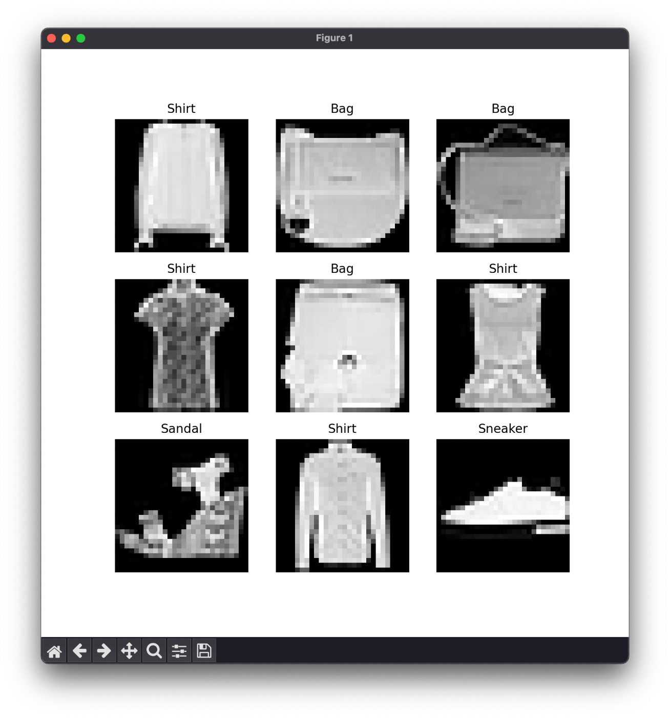
実行結果
Iterate through the DataLoader
train_dataloader = DataLoader(training_data, batch_size=64, shuffle=True)
test_dataloader = DataLoader(test_data, batch_size=64, shuffle=True)

train_features, train_labels = next(iter(train_dataloader))
print(f"Feature batch shape: {train_features.size()}")
print(f"Labels batch shape: {train_labels.size()}")
img = train_features[0].squeeze()
label = train_labels[0]
plt.imshow(img, cmap="gray")
plt.show()
print(f"Label: {label}")
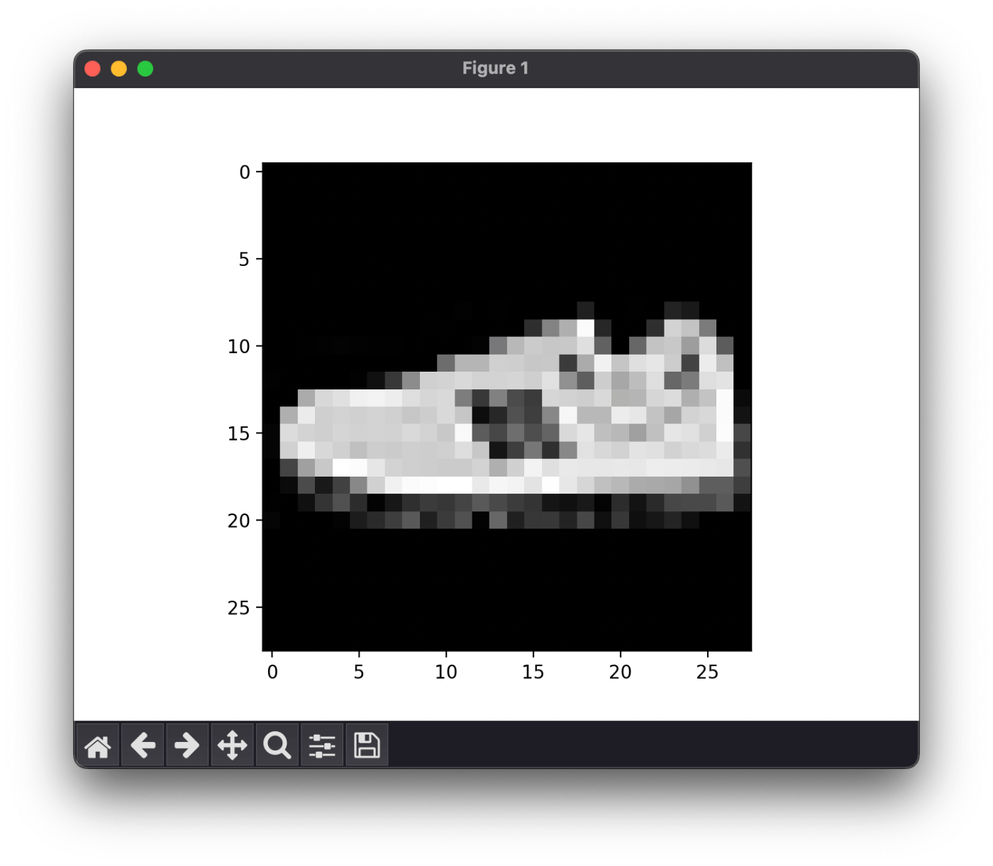
実行結果
Feature batch shape: torch.Size([64, 1, 28, 28])
Labels batch shape: torch.Size([64])
Label: 7
squeeze() って何?
> x = np.array([[[0], [1], [2]]])
> x.shape
(1, 3, 1)
> np.squeeze(x).shape
(3,)
余計な [] を取り除いてくれるようだ。
データセットページの所要時間
途中端折ったので 30 分くらいかな。
次はトランスフォームを読もう。
scatter() メソッド
self[index[i]] = src[i] # if dim == 0
self[index[i][j]][j] = src[i][j]  # if dim == 0
self[i][index[i][j]] = src[i][j]  # if dim == 1
self[index[i][j][k]][j][k] = src[i][j][k]  # if dim == 0
self[i][index[i][j][k]][k] = src[i][j][k]  # if dim == 1
self[i][j][index[i][j][k]] = src[i][j][k]  # if dim == 2
>>> src = torch.arange(1, 11).reshape((2, 5))
>>> src
tensor([[ 1,  2,  3,  4,  5],
        [ 6,  7,  8,  9, 10]])
>>> index = torch.tensor([[0, 1, 2, 0]])
>>> torch.zeros(3, 5, dtype=src.dtype).scatter_(0, index, src)
tensor([[1, 0, 0, 4, 0],
        [0, 2, 0, 0, 0],
        [0, 0, 3, 0, 0]])
>>> index = torch.tensor([[0, 1, 2], [0, 1, 4]])
>>> torch.zeros(3, 5, dtype=src.dtype).scatter_(1, index, src)
tensor([[1, 2, 3, 0, 0],
        [6, 7, 0, 0, 8],
        [0, 0, 0, 0, 0]])

>>> torch.full((2, 4), 2.).scatter_(1, torch.tensor([[2], [3]]),
...            1.23, reduce='multiply')
tensor([[2.0000, 2.0000, 2.4600, 2.0000],
        [2.0000, 2.0000, 2.0000, 2.4600]])
>>> torch.full((2, 4), 2.).scatter_(1, torch.tensor([[2], [3]]),
...            1.23, reduce='add')
tensor([[2.0000, 2.0000, 3.2300, 2.0000],
        [2.0000, 2.0000, 2.0000, 3.2300]])
うまく説明できないけどやっていることはわかる気がする。
Lambda Transforms
touch transforms.py
import torch


def target_transform_lambda(y):
    zeros = torch.zeros(10, dtype=torch.float)
    return zeros.scatter_(dim=0, index=torch.tensor(y), value=1)


print(target_transform_lambda(0))
print(target_transform_lambda(1))
print(target_transform_lambda(9))
tensor([1., 0., 0., 0., 0., 0., 0., 0., 0., 0.])
tensor([0., 1., 0., 0., 0., 0., 0., 0., 0., 0.])
tensor([0., 0., 0., 0., 0., 0., 0., 0., 0., 1.])
トランスフォームとして使うには from torchvision.transforms import Lambda が必要になる。
なんだかんだで 30 分くらいかかった
次はニューラルネットワーク作成のページを読む。
転移学習とファインチューニング
事前に学習したモデルに出力層を追加する手法とのことらしい。
転移学習ではモデルのパラメータを固定するが、ファインチューニングではモデルのパラメータも更新するようだ。
5/22 (月) はここから
このスクラップの目標は ResNet などの既存モデルを使って転移学習で物体検出を行うことに設定してみよう。
難しければもう少しレベルを下げてみよう。
PyTorch の読み方とライセンス
パイトーチが多数派なのかな?
ライセンスは BSD スタイルのようだがなんか注意があるように聞いた。
ONNX も気になる
共通のデータフォーマットのようだ。
転移学習のチュートリアルをやってみよう
ファインチューニングは転移学習の一種
転移学習だと思っていたものは特徴抽出(feature extractor)と呼ばれるようだ。
このチュートリアルでやること
アリとハチを分類するみたいだ。
データは下記からダウンロードする、サイズは 40 MB ほど。
ダウンロードしたワークスペースに data/hymenoptera_data として展開する。
ソースコード作成
touch transfer-learning.py
画像の読み込み
import os
import torch
import torch.utils.data
from torchvision import datasets, transforms

data_transforms = {
    'train': transforms.Compose([
        transforms.RandomResizedCrop(224),
        transforms.RandomHorizontalFlip(),
        transforms.ToTensor(),
        transforms.Normalize([0.485, 0.456, 0.406], [0.229, 0.224, 0.225])
    ]),
    'val': transforms.Compose([
        transforms.Resize(256),
        transforms.CenterCrop(224),
        transforms.ToTensor(),
        transforms.Normalize([0.485, 0.456, 0.406], [0.229, 0.224, 0.225])
    ]),
}

data_dir = 'data/hymenoptera_data'
image_datasets = {
    x: datasets.ImageFolder(
        os.path.join(data_dir, x), data_transforms[x])
    for x in ['train', 'val']
}

dataloaders = {
    x: torch.utils.data.DataLoader(
        image_datasets[x],
        batch_size=4,
        shuffle=True,
        num_workers=4)
    for x in ['train', 'val']
}

dataset_sizes = {
    x: len(image_datasets[x]) for x in ['train', 'val']
}

class_names = image_datasets['train'].classes

device = torch.device('cpu')

print(dataset_sizes)
print(class_names)
{'train': 244, 'val': 153}
['ants', 'bees']
データの可視化
import os
from matplotlib import pyplot as plt
import numpy as np
import torch
import torch.utils.data
from torchvision import datasets, transforms
import torchvision.utils

data_transforms = {
    'train': transforms.Compose([
        transforms.RandomResizedCrop(224),
        transforms.RandomHorizontalFlip(),
        transforms.ToTensor(),
        transforms.Normalize([0.485, 0.456, 0.406], [0.229, 0.224, 0.225])
    ]),
    'val': transforms.Compose([
        transforms.Resize(256),
        transforms.CenterCrop(224),
        transforms.ToTensor(),
        transforms.Normalize([0.485, 0.456, 0.406], [0.229, 0.224, 0.225])
    ]),
}

data_dir = 'data/hymenoptera_data'
image_datasets = {
    x: datasets.ImageFolder(
        os.path.join(data_dir, x), data_transforms[x])
    for x in ['train', 'val']
}

dataloaders = {
    x: torch.utils.data.DataLoader(
        image_datasets[x],
        batch_size=4,
        shuffle=True,
        num_workers=4)
    for x in ['train', 'val']
}

dataset_sizes = {
    x: len(image_datasets[x]) for x in ['train', 'val']
}

class_names = image_datasets['train'].classes

device = torch.device('cpu')

# print(dataset_sizes)
# print(class_names)


def imshow(inp: torch.Tensor, title=None):
    inp = inp.numpy().transpose((1, 2, 0))
    mean = np.array([0.485, 0.456, 0.406])
    std = np.array([0.229, 0.224, 0.225])
    inp = std * inp + mean
    inp = np.clip(inp, 0, 1)
    plt.imshow(inp)
    if title is not None:
        plt.title(title)
    # plt.pause(0.001)
    plt.show()


if __name__ == "__main__":
    inputs, classes = next(iter(dataloaders['train']))
    out = torchvision.utils.make_grid(inputs)
    imshow(out, title=[class_names[x] for x in classes])
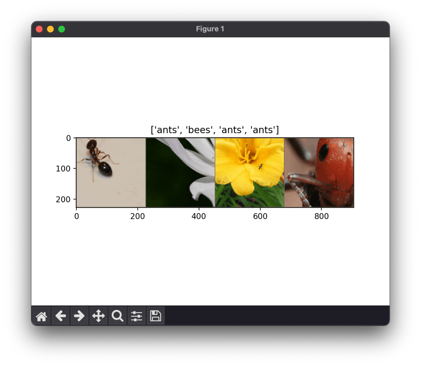
表示されたグラフ
Transpose って何?
転置するようだ。
make_grid って何?
複数の画像を並べた画像を生成するようだ。
(B, C, H, W) → (C, H', W') に変換するので転置が必要だったようだ。
H' と W' は枠線が入ったり並べたりする関係で増える。
5/22 (月) はここまで
ここまでの作業時間は 1.25 時間くらい。
そのうちどのチュートリアルをするかを調べた時間が 0.5 時間くらい。
5/23 (火) はここから
チュートリアルを進めたい、完了は難しいだろうな。
train_model() 関数の写経
def train_model(model, criterion, optimizer, scheduler, num_epochs=25):
    since = time.time()

    best_model_wts = copy.deepcopy(model.state_dict())
    best_acc = 0.0

    for epoch in range(num_epochs):
        print(f"Epoch {epoch}/{num_epochs - 1}")
        print('-' * 10)

        for phase in ['train', 'val']:
            if phase == 'train':
                model.train()
            else:
                model.eval()

            running_loss = 0.0
            running_corrects = 0

            for inputs, labels in dataloaders[phase]:
                inputs = inputs.to(device)
                labels = labels.to(device)

                optimizer.zero_grad()

                with torch.set_grad_enabled(phase == 'train'):
                    outputs = model(inputs)
                    _, preds = torch.max(outputs, 1)
                    loss = criterion(outputs, labels)

                    if phase == 'train':
                        loss.backward()
                        optimizer.step()

                running_loss += loss.item() * inputs.size(0)
                running_corrects += torch.sum(preds == labels.data)
            if phase == 'train':
                scheduler.step()

            epoch_loss = running_loss / dataset_sizes[phase]
            epoch_acc = running_corrects.double() / dataset_sizes[phase]

            print(f'{phase} Loss: {epoch_loss:.4f} Acc: {epoch_acc:.4f}')

            if phase == 'val' and epoch_acc > best_acc:
                best_acc = epoch_acc
                best_model_wts = copy.deepcopy(model.state_dict())

        print()

        time_elapsed = time.time() - since
        print(
            f'Training complete in {time_elapsed // 60:.0f}m {time_elapsed % 60:.0f}s')
        print(f'Best val Acc: {best_acc:4f}')

        model.load_state_dict(best_model_wts)
        return model
何をやっているのかわかるようなわからないような。
あと何回か写経しないと何やっているかが体得できなそうだ。
visualize_model() の写経
def visualize_model(model, num_images=6):
    was_training = model.training
    model.eval()
    images_so_far = 0
    fig = plt.figure()

    with torch.no_grad():
        for i, (inputs, labels) in enumerate(dataloaders['val']):
            inputs = inputs.to(device)
            labels = labels.to(device)

            outputs = model(inputs)

            # torch.max() 関数の第 2 引数は最大値を計算する次元
            # 戻り値はタプルで第 1 要素が値で第 2 要素がインデックス
            # https://pytorch.org/docs/stable/generated/torch.max.html#torch.max
            _, preds = torch.max(outputs, 1)

            for j in range(input.size()[0]):
                images_so_far += 1
                ax = plt.subplot(num_images // 2, 2, images_so_far)
                ax.axis('off')
                ax.set_title(f'predicated: {class_names[preds[j]]}')
                imshow(inputs.cpu().data[j])

                if images_so_far == num_images:
                    model.train(mode=was_training)
                    return
            model.train(mode=was_training)
なんというか、ステップバイステップで確認しながら進められると嬉しいのだがチュートリアルに文句を言っても仕方がない。
ファインチューニングの写経
model_ft = models.resnet18(weights='IMAGENET1K_V1')
num_ftrs = model_ft.fc.in_features
model_ft.fc = nn.Linear(num_ftrs, 2)
model_ft = model_ft.to(device)

criterion = nn.CrossEntropyLoss()
optimizer_ft = optim.SGD(model_ft.parameters(), lr=0.001, momentum=0.9)
exp_lr_scheduler = lr_scheduler.StepLR(optimizer_ft, step_size=7, gamma=0.1)
この部分はなんとなくやっていることがわかる気がする。
ファインチューニングする場合は最後の層を置き換えれば良いんだね。
学習と評価
エポック数が 25 だと CPU の場合に学習時間が 15〜25 分になるようなのでまずは 1 とした。
if __name__ == '__main__':
    model_ft = train_model(model_ft, criterion, optimizer_ft,
                           exp_lr_scheduler, num_epochs=1)
    visualize_model(model_ft)
if __name__ == '__main__': がないとマルチプロセスの関係で例外が発生する。
警告表示
学習時も評価時も下記のような警告が 4 件ずつ表示される。
[W ParallelNative.cpp:230] Warning: Cannot set number of intraop threads after parallel work has started or after set_num_threads call when using native parallel backend (function set_num_threads)
モデルの可視化
実行してから 1〜2 分かかってやっと表示される。
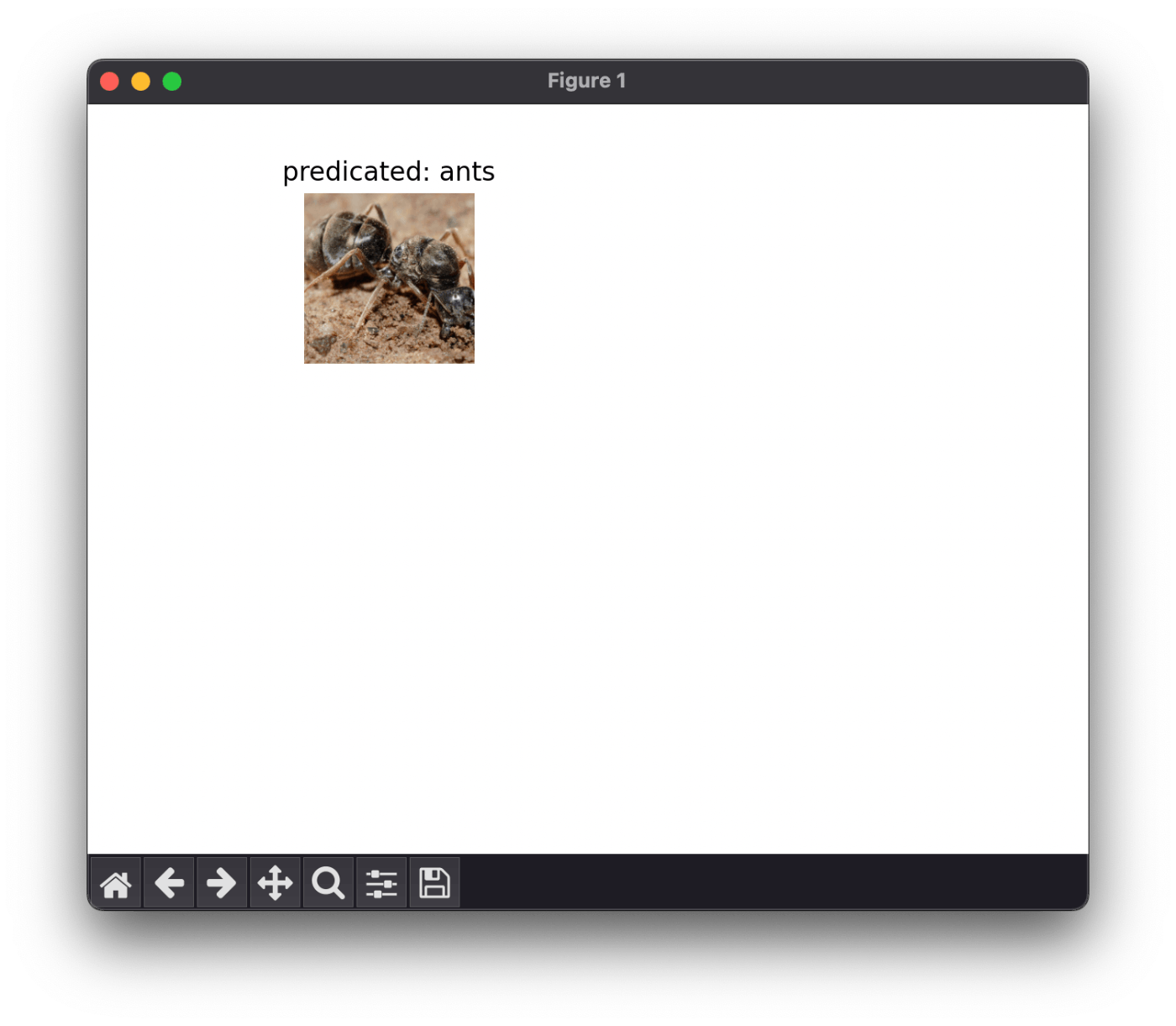
なぜか 1 枚しか表示されない
ResNet を特徴抽出器として使う
# model_ft = models.resnet18(weights='IMAGENET1K_V1')
# num_ftrs = model_ft.fc.in_features
# model_ft.fc = nn.Linear(num_ftrs, 2)
# model_ft = model_ft.to(device)

# criterion = nn.CrossEntropyLoss()
# optimizer_ft = optim.SGD(model_ft.parameters(), lr=0.001, momentum=0.9)
# exp_lr_scheduler = lr_scheduler.StepLR(optimizer_ft, step_size=7, gamma=0.1)

# if __name__ == '__main__':
#     model_ft = train_model(model_ft, criterion, optimizer_ft,
#                            exp_lr_scheduler, num_epochs=1)
#     visualize_model(model_ft)


model_conv = models.resnet18(weights='IMAGENET1K_V1')
for param in model_conv.parameters():
    param.requires_grad = False

num_ftrs = model_conv.fc.in_features
model_conv.fc = nn.Linear(num_ftrs, 2)
model_conv = model_conv.to(device)

criterion = nn.CrossEntropyLoss()
optimizer_ft = optim.SGD(model_conv.fc.parameters(), lr=0.001, momentum=0.9)
exp_lr_scheduler = lr_scheduler.StepLR(optimizer_ft, step_size=7, gamma=0.1)

if __name__ == '__main__':
    model_ft = train_model(model_conv, criterion, optimizer_ft,
                           exp_lr_scheduler, num_epochs=1)
    visualize_model(model_ft)
こちらも最後の層を付け替えている。
パラメーターの requires_grald を False にする手続きが追加されている点や、SGD の第 1 引数が model_conv.fc.parameters() となっている点がファインチューニングとは異なる。
モデルの可視化
特徴抽出の場合も結構時間がかかるがファインチューニングよりも短い。
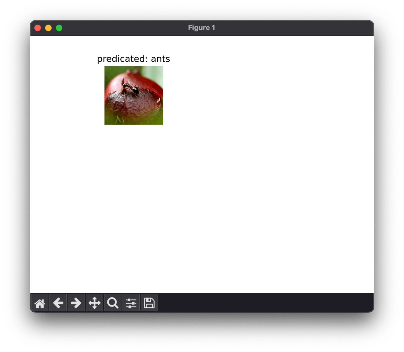
相変わらず 1 枚しか表示されない
コンソール出力の比較
Epoch 0/0
----------
train Loss: 0.5992 Acc: 0.6885
val Loss: 0.2641 Acc: 0.9020

Training complete in 1m 34s
Best val Acc: 0.901961
Epoch 0/0
----------
train Loss: 0.5322 Acc: 0.7049
val Loss: 0.2668 Acc: 0.8889

Training complete in 1m 10s
Best val Acc: 0.888889
たしかに特徴抽出の方が実行時間は短い。
評価についてはエポックが 1 回だけで運要素満載なので特に考察することはない。
5/23 (火) はここまで
ちょうど 1 時間くらい経ったかな。
とりあえずファインチューニングを動かせて良かった。
全く理解していないがいずれ理解できる時が来るだろう、少なくとも使い方くらいは。
集計していないけど今のところ 6 時間くらいかな?
ドキュメントを読んでいる時間も含めると既に 8 時間くらい投資している気がする。
なかなか PyTorch に慣れないが着実に進めていると信じたい。
サンプルソースを見ないで使えるレベルにはなりたい、欲を言えば何をやっているのかを知りたい。
クローズする前に 1 回だけ復習しよう。
5/24 (水) はここから
そろそろ Jupyter Notebook の使い方でも学ぶか。
Jupyter Notebook のインストール
pip install notebook
Jupyter Notebook 起動
# cd ~/workspace/python/hello-pytorch
jupyter notebook
自動的に http://localhost:8888/tree が開く
ノートブックの作成
右上のボタンから新規 > Python 3 を選ぶ。

ノートブックが作成された
自動補完
下記で設定できるようだ。
pip install jupyter-contrib-nbextensions
pip install jupyter-nbextensions-configurator
jupyter contrib nbextension install
jupyter nbextensions_configurator enable
もしかして JupyterLab 使った方が良い?
pip install jupyterlab
jupyter-lab

JupyterLab の方がカッコ良い
Tab で自動補完が効く

VSCode が凄すぎて物足りない
JupyterLab の対話的に実行できるのは素晴らしいが VSCode のコーディング支援が凄すぎて物足りなさを感じる。
使い分け次第だが基本は VSCode でコーディングした方が捗りそう。
5/24 (水) はここまで
30 分くらい学んだ、今のところ 6.5 時間くらいか。
明日は物体検出でもやってみようかな。
5/25 (木) はここから
今日は疲れて物体検出をやる元気がないので初心に帰って復習をしよう。
QuickStart Again
touch quickstart_again.py
寄り道しながらやっていこう。
データセットの寄り道
from torchvision import datasets
from torchvision.transforms import ToTensor

# Fasion MNIST のデータセットを取得します。
training_data = datasets.FashionMNIST(
    root="data",
    train=True,
    download=True,
    transform=ToTensor(),
)

# データ件数を表示します。
print(training_data.__len__())

# 1 件目のデータを取得します。
print(training_data.__getitem__(0))
60000
(tensor([[[0.0000, 0.0000, 0.0000, 0.0000, 0.0000, 0.0000, 0.0000, 0.0000,
          0.0000, 0.0000, 0.0000, 0.0000, 0.0000, 0.0000, 0.0000, 0.0000,
          0.0000, 0.0000, 0.0000, 0.0000, 0.0000, 0.0000, 0.0000, 0.0000,
          0.0000, 0.0000, 0.0000, 0.0000],
         [0.0000, 0.0000, 0.0000, 0.0000, 0.0000, 0.0000, 0.0000, 0.0000,
          0.0000, 0.0000, 0.0000, 0.0000, 0.0000, 0.0000, 0.0000, 0.0000,
          0.0000, 0.0000, 0.0000, 0.0000, 0.0000, 0.0000, 0.0000, 0.0000,
          0.0000, 0.0000, 0.0000, 0.0000],
         [0.0000, 0.0000, 0.0000, 0.0000, 0.0000, 0.0000, 0.0000, 0.0000,
          0.0000, 0.0000, 0.0000, 0.0000, 0.0000, 0.0000, 0.0000, 0.0000,
          0.0000, 0.0000, 0.0000, 0.0000, 0.0000, 0.0000, 0.0000, 0.0000,
          0.0000, 0.0000, 0.0000, 0.0000],
         [0.0000, 0.0000, 0.0000, 0.0000, 0.0000, 0.0000, 0.0000, 0.0000,
          0.0000, 0.0000, 0.0000, 0.0000, 0.0039, 0.0000, 0.0000, 0.0510,
          0.2863, 0.0000, 0.0000, 0.0039, 0.0157, 0.0000, 0.0000, 0.0000,
          0.0000, 0.0039, 0.0039, 0.0000],
         [0.0000, 0.0000, 0.0000, 0.0000, 0.0000, 0.0000, 0.0000, 0.0000,
          0.0000, 0.0000, 0.0000, 0.0000, 0.0118, 0.0000, 0.1412, 0.5333,
          0.4980, 0.2431, 0.2118, 0.0000, 0.0000, 0.0000, 0.0039, 0.0118,
          0.0157, 0.0000, 0.0000, 0.0118],
         [0.0000, 0.0000, 0.0000, 0.0000, 0.0000, 0.0000, 0.0000, 0.0000,
          0.0000, 0.0000, 0.0000, 0.0000, 0.0235, 0.0000, 0.4000, 0.8000,
          0.6902, 0.5255, 0.5647, 0.4824, 0.0902, 0.0000, 0.0000, 0.0000,
          0.0000, 0.0471, 0.0392, 0.0000],
         [0.0000, 0.0000, 0.0000, 0.0000, 0.0000, 0.0000, 0.0000, 0.0000,
          0.0000, 0.0000, 0.0000, 0.0000, 0.0000, 0.0000, 0.6078, 0.9255,
          0.8118, 0.6980, 0.4196, 0.6118, 0.6314, 0.4275, 0.2510, 0.0902,
          0.3020, 0.5098, 0.2824, 0.0588],
         [0.0000, 0.0000, 0.0000, 0.0000, 0.0000, 0.0000, 0.0000, 0.0000,
          0.0000, 0.0000, 0.0000, 0.0039, 0.0000, 0.2706, 0.8118, 0.8745,
          0.8549, 0.8471, 0.8471, 0.6392, 0.4980, 0.4745, 0.4784, 0.5725,
          0.5529, 0.3451, 0.6745, 0.2588],
         [0.0000, 0.0000, 0.0000, 0.0000, 0.0000, 0.0000, 0.0000, 0.0000,
          0.0000, 0.0039, 0.0039, 0.0039, 0.0000, 0.7843, 0.9098, 0.9098,
          0.9137, 0.8980, 0.8745, 0.8745, 0.8431, 0.8353, 0.6431, 0.4980,
          0.4824, 0.7686, 0.8980, 0.0000],
         [0.0000, 0.0000, 0.0000, 0.0000, 0.0000, 0.0000, 0.0000, 0.0000,
          0.0000, 0.0000, 0.0000, 0.0000, 0.0000, 0.7176, 0.8824, 0.8471,
          0.8745, 0.8941, 0.9216, 0.8902, 0.8784, 0.8706, 0.8784, 0.8667,
          0.8745, 0.9608, 0.6784, 0.0000],
         [0.0000, 0.0000, 0.0000, 0.0000, 0.0000, 0.0000, 0.0000, 0.0000,
          0.0000, 0.0000, 0.0000, 0.0000, 0.0000, 0.7569, 0.8941, 0.8549,
          0.8353, 0.7765, 0.7059, 0.8314, 0.8235, 0.8275, 0.8353, 0.8745,
          0.8627, 0.9529, 0.7922, 0.0000],
         [0.0000, 0.0000, 0.0000, 0.0000, 0.0000, 0.0000, 0.0000, 0.0000,
          0.0000, 0.0039, 0.0118, 0.0000, 0.0471, 0.8588, 0.8627, 0.8314,
          0.8549, 0.7529, 0.6627, 0.8902, 0.8157, 0.8549, 0.8784, 0.8314,
          0.8863, 0.7725, 0.8196, 0.2039],
         [0.0000, 0.0000, 0.0000, 0.0000, 0.0000, 0.0000, 0.0000, 0.0000,
          0.0000, 0.0000, 0.0235, 0.0000, 0.3882, 0.9569, 0.8706, 0.8627,
          0.8549, 0.7961, 0.7765, 0.8667, 0.8431, 0.8353, 0.8706, 0.8627,
          0.9608, 0.4667, 0.6549, 0.2196],
         [0.0000, 0.0000, 0.0000, 0.0000, 0.0000, 0.0000, 0.0000, 0.0000,
          0.0000, 0.0157, 0.0000, 0.0000, 0.2157, 0.9255, 0.8941, 0.9020,
          0.8941, 0.9412, 0.9098, 0.8353, 0.8549, 0.8745, 0.9176, 0.8510,
          0.8510, 0.8196, 0.3608, 0.0000],
         [0.0000, 0.0000, 0.0039, 0.0157, 0.0235, 0.0275, 0.0078, 0.0000,
          0.0000, 0.0000, 0.0000, 0.0000, 0.9294, 0.8863, 0.8510, 0.8745,
          0.8706, 0.8588, 0.8706, 0.8667, 0.8471, 0.8745, 0.8980, 0.8431,
          0.8549, 1.0000, 0.3020, 0.0000],
         [0.0000, 0.0118, 0.0000, 0.0000, 0.0000, 0.0000, 0.0000, 0.0000,
          0.0000, 0.2431, 0.5686, 0.8000, 0.8941, 0.8118, 0.8353, 0.8667,
          0.8549, 0.8157, 0.8275, 0.8549, 0.8784, 0.8745, 0.8588, 0.8431,
          0.8784, 0.9569, 0.6235, 0.0000],
         [0.0000, 0.0000, 0.0000, 0.0000, 0.0706, 0.1725, 0.3216, 0.4196,
          0.7412, 0.8941, 0.8627, 0.8706, 0.8510, 0.8863, 0.7843, 0.8039,
          0.8275, 0.9020, 0.8784, 0.9176, 0.6902, 0.7373, 0.9804, 0.9725,
          0.9137, 0.9333, 0.8431, 0.0000],
         [0.0000, 0.2235, 0.7333, 0.8157, 0.8784, 0.8667, 0.8784, 0.8157,
          0.8000, 0.8392, 0.8157, 0.8196, 0.7843, 0.6235, 0.9608, 0.7569,
          0.8078, 0.8745, 1.0000, 1.0000, 0.8667, 0.9176, 0.8667, 0.8275,
          0.8627, 0.9098, 0.9647, 0.0000],
         [0.0118, 0.7922, 0.8941, 0.8784, 0.8667, 0.8275, 0.8275, 0.8392,
          0.8039, 0.8039, 0.8039, 0.8627, 0.9412, 0.3137, 0.5882, 1.0000,
          0.8980, 0.8667, 0.7373, 0.6039, 0.7490, 0.8235, 0.8000, 0.8196,
          0.8706, 0.8941, 0.8824, 0.0000],
         [0.3843, 0.9137, 0.7765, 0.8235, 0.8706, 0.8980, 0.8980, 0.9176,
          0.9765, 0.8627, 0.7608, 0.8431, 0.8510, 0.9451, 0.2549, 0.2863,
          0.4157, 0.4588, 0.6588, 0.8588, 0.8667, 0.8431, 0.8510, 0.8745,
          0.8745, 0.8784, 0.8980, 0.1137],
         [0.2941, 0.8000, 0.8314, 0.8000, 0.7569, 0.8039, 0.8275, 0.8824,
          0.8471, 0.7255, 0.7725, 0.8078, 0.7765, 0.8353, 0.9412, 0.7647,
          0.8902, 0.9608, 0.9373, 0.8745, 0.8549, 0.8314, 0.8196, 0.8706,
          0.8627, 0.8667, 0.9020, 0.2627],
         [0.1882, 0.7961, 0.7176, 0.7608, 0.8353, 0.7725, 0.7255, 0.7451,
          0.7608, 0.7529, 0.7922, 0.8392, 0.8588, 0.8667, 0.8627, 0.9255,
          0.8824, 0.8471, 0.7804, 0.8078, 0.7294, 0.7098, 0.6941, 0.6745,
          0.7098, 0.8039, 0.8078, 0.4510],
         [0.0000, 0.4784, 0.8588, 0.7569, 0.7020, 0.6706, 0.7176, 0.7686,
          0.8000, 0.8235, 0.8353, 0.8118, 0.8275, 0.8235, 0.7843, 0.7686,
          0.7608, 0.7490, 0.7647, 0.7490, 0.7765, 0.7529, 0.6902, 0.6118,
          0.6549, 0.6941, 0.8235, 0.3608],
         [0.0000, 0.0000, 0.2902, 0.7412, 0.8314, 0.7490, 0.6863, 0.6745,
          0.6863, 0.7098, 0.7255, 0.7373, 0.7412, 0.7373, 0.7569, 0.7765,
          0.8000, 0.8196, 0.8235, 0.8235, 0.8275, 0.7373, 0.7373, 0.7608,
          0.7529, 0.8471, 0.6667, 0.0000],
         [0.0078, 0.0000, 0.0000, 0.0000, 0.2588, 0.7843, 0.8706, 0.9294,
          0.9373, 0.9490, 0.9647, 0.9529, 0.9569, 0.8667, 0.8627, 0.7569,
          0.7490, 0.7020, 0.7137, 0.7137, 0.7098, 0.6902, 0.6510, 0.6588,
          0.3882, 0.2275, 0.0000, 0.0000],
         [0.0000, 0.0000, 0.0000, 0.0000, 0.0000, 0.0000, 0.0000, 0.1569,
          0.2392, 0.1725, 0.2824, 0.1608, 0.1373, 0.0000, 0.0000, 0.0000,
          0.0000, 0.0000, 0.0000, 0.0000, 0.0000, 0.0000, 0.0000, 0.0000,
          0.0000, 0.0000, 0.0000, 0.0000],
         [0.0000, 0.0000, 0.0000, 0.0000, 0.0000, 0.0000, 0.0000, 0.0000,
          0.0000, 0.0000, 0.0000, 0.0000, 0.0000, 0.0000, 0.0000, 0.0000,
          0.0000, 0.0000, 0.0000, 0.0000, 0.0000, 0.0000, 0.0000, 0.0000,
          0.0000, 0.0000, 0.0000, 0.0000],
         [0.0000, 0.0000, 0.0000, 0.0000, 0.0000, 0.0000, 0.0000, 0.0000,
          0.0000, 0.0000, 0.0000, 0.0000, 0.0000, 0.0000, 0.0000, 0.0000,
          0.0000, 0.0000, 0.0000, 0.0000, 0.0000, 0.0000, 0.0000, 0.0000,
          0.0000, 0.0000, 0.0000, 0.0000]]]), 9)
テンソルの形の確認
tensor, label = training_data.__getitem__(0)
print(tensor.shape)
torch.Size([1, 28, 28])
テンソルの形の確認
# データを画像で表示します。
# tensor の形状は (C, H, W) であるのに対し、
# imshow の引数の形状は (H, W, C) です。
# 形状を合わせるために torch.permute() 関数を使っています。
plt.imshow(torch.permute(tensor, (1, 2, 0)))
plt.show()

表示される画像
下記を参考にした。
DataLoader の使用
from matplotlib import pyplot as plt
import torch
from torch.utils.data import DataLoader
from torchvision import datasets
from torchvision.transforms import ToTensor

# Fasion MNIST のデータセットを取得します。
training_data = datasets.FashionMNIST(
    root="data",
    train=True,
    download=True,
    transform=ToTensor(),
)

test_data = datasets.FashionMNIST(
    root="data",
    train=False,
    download=True,
    transform=ToTensor(),
)

# データ件数を表示します。
# print(training_data.__len__())
# print(test_data.__len__())

# 1 件目のデータを取得します。
# print(training_data.__getitem__(0))
# print(test_data.__getitem__(0))

# データの形状を表示します。
# training_tensor, label = training_data.__getitem__(0)
# test_tensor, label = test_data.__getitem__(0)
# print(training_tensor.shape)
# print(test_tensor.shape)

# データを画像で表示します。
# tensor の形状は (C, H, W) であるのに対し、
# imshow の引数の形状は (H, W, C) です。
# 形状を合わせるために torch.permute() 関数を使っています。
# plt.imshow(torch.permute(test_tensor, (1, 2, 0)))
# plt.show()

batch_size = 64
train_dataloader = DataLoader(training_data, batch_size=batch_size)
test_dataloader = DataLoader(test_data, batch_size=batch_size)

# 評価用のデータとラベルを batch_size の数だけ読み込みます。
for X, y in test_dataloader:
    print(X.shape)
    print(y.shape)
    print(y.dtype)
    break
torch.Size([64, 1, 28, 28])
torch.Size([64])
torch.int64
こういうのをミニバッチと呼ぶんだっけ?
DataLoader については色々なオプションがあって興味深いが基本的な機能はデータセットから for ループでデータとラベルを取得できるようにすることと理解している。
5/25 (木) はここまで
復習なので色々と気になることを試せて楽しい。
torch.permute() 関数についても知れて良かった、これでいつでも画像が表示できる。
明日も復習を続けよう。
今日も 30 分くらい学んだので累計で 7 時間くらいか。
5/26 (金) はここから
ちょっと早起きしたので 30 分くらいやろうかな。
モデル作成
device = "cpu"


class NeuralNetwork(nn.Module):
    def __init__(self):
        super().__init__()
        self.flatten = nn.Flatten()
        self.linear_relu_stack = nn.Sequential(
            nn.Linear(28 * 28, 512),
            nn.ReLU(),
            nn.Linear(512, 512),
            nn.ReLU(),
            nn.Linear(512, 10),
        )

    def forward(self, x):
        x = self.flatten(x)
        logits = self.linear_relu_stack(x)
        return logits


model = NeuralNetwork().to(device)
print(model)
NeuralNetwork(
  (flatten): Flatten(start_dim=1, end_dim=-1)
  (linear_relu_stack): Sequential(
    (0): Linear(in_features=784, out_features=512, bias=True)
    (1): ReLU()
    (2): Linear(in_features=512, out_features=512, bias=True)
    (3): ReLU()
    (4): Linear(in_features=512, out_features=10, bias=True)
  )
)
logits とはなんだろうと思って調べたところオッズ p / (1 - p) の対数のようだ。
パラメーターの表示
loss_fn = nn.CrossEntropyLoss()
parameters = model.parameters()

# パラメータの内容を表示します。
print(next(parameters).shape)
print(next(parameters).shape)
print(next(parameters).shape)
print(next(parameters).shape)
print(next(parameters).shape)
print(next(parameters).shape)
optimizer = torch.optim.SGD(parameters, lr=1e-3)
torch.Size([512, 784])
torch.Size([512])
torch.Size([512, 512])
torch.Size([512])
torch.Size([10, 512])
torch.Size([10])
想像するに奇数番号は y = Ax + b の A の部分で偶数番号は b の部分なのだろう。
テンソルの形状は (出力数、入力数) になっている。
交差エントロピー誤差については下記の記事がわかりやすい。
SGD については確率的勾配降下法のことらしい。
学習
size = len(train_dataloader.dataset)
model.train()
for batch, (X, y) in enumerate(train_dataloader):
    X, y = X.to(device), y.to(device)

    pred = model(X)
    loss = loss_fn(pred, y)

    # この 3 行がよくわからない
    loss.backward()
    optimizer.step()
    optimizer.zero_grad()

    if batch % 100 == 0:
        loss, current = loss.item(), (batch + 1) * len(X)
        print(f"loss: {loss:>7f} [{current:>5d}/{size:>5d}]")
30 分経ってしまったので後からよくわからない 3 行について調べよう。
勉強になります
5/27 (土) はここから
気晴らしに 30 分くらい勉強しよう。
loss.backward() と optimizer.step()
おそらく前者は偏微分を計算し、後者はパラメーターを調整している。
そう辺りをつけた上で調べてみよう。
こちらの記事がとてもわかりやすい
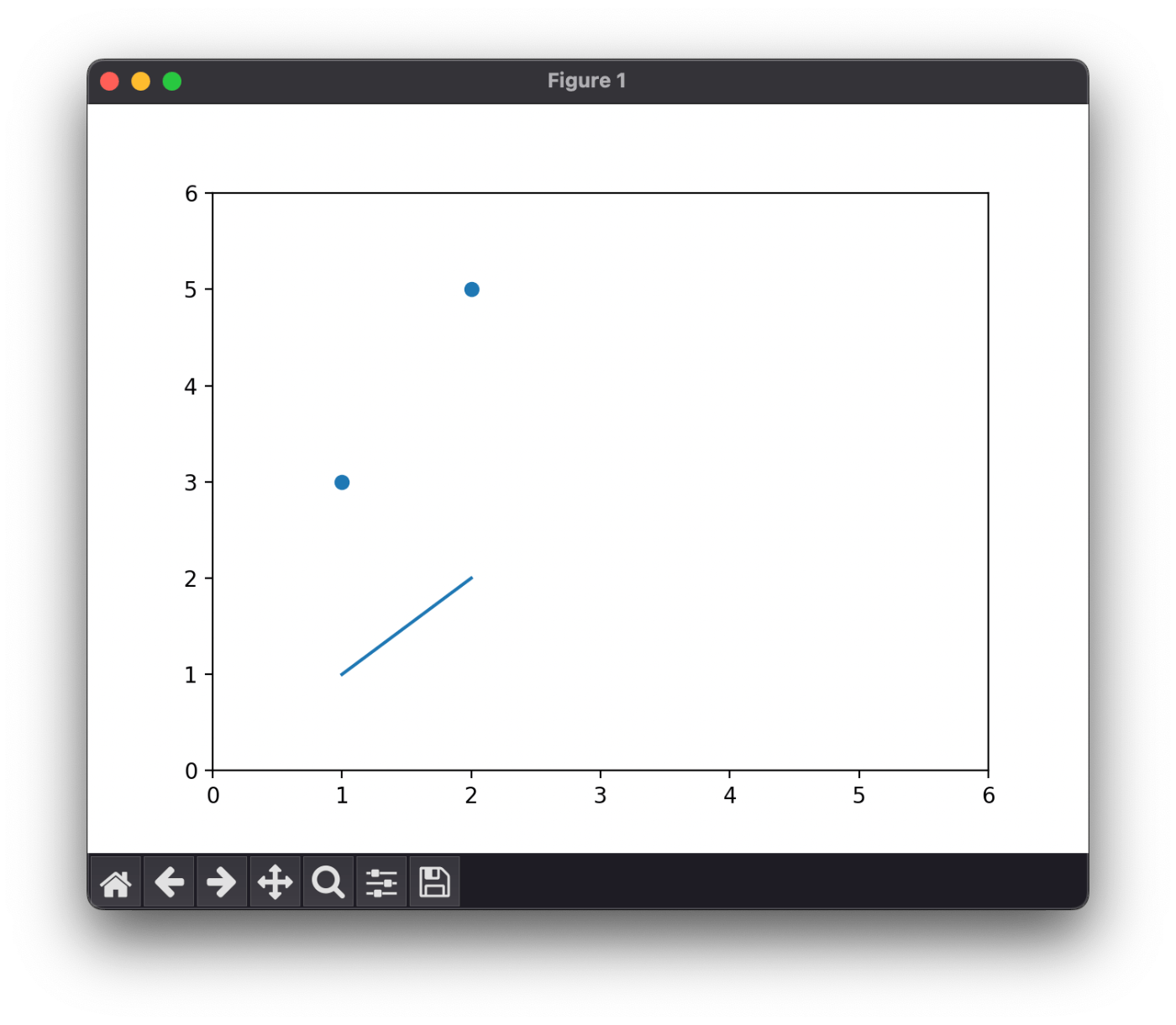
体感してみる
touch backward.py
from matplotlib import pyplot as plt
import torch


x = torch.Tensor([1, 2])
t = torch.Tensor([3, 5])

plt.scatter(x, t)
plt.xlim((0, 6))
plt.ylim((0, 6))
plt.show()
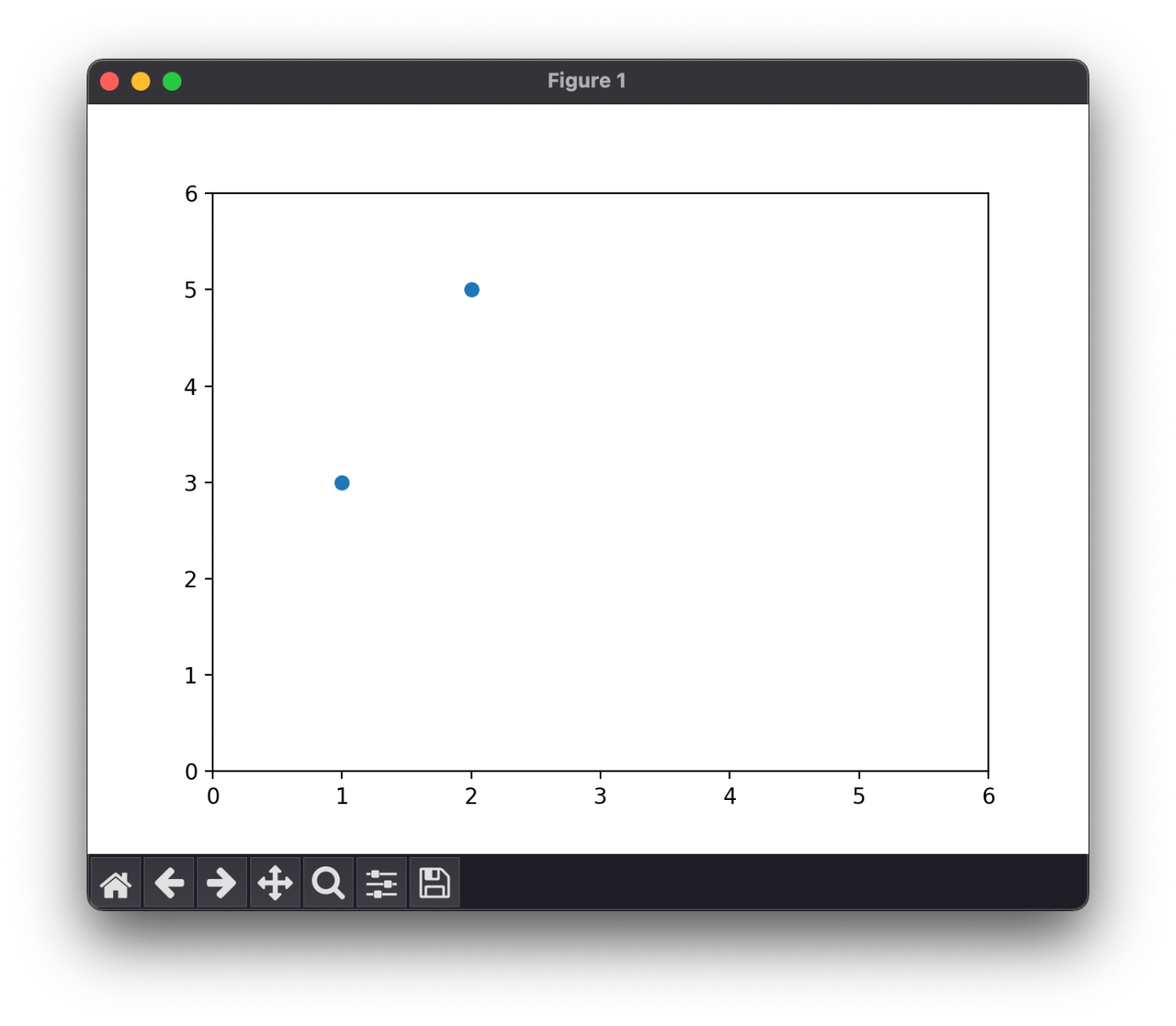
出力されるグラフ
勾配の表示
# 適当にパラメータを決める
a = torch.tensor(1., requires_grad=True)
b = torch.tensor(0., requires_grad=True)
print(a.grad, b.grad)
None None
誤差の表示
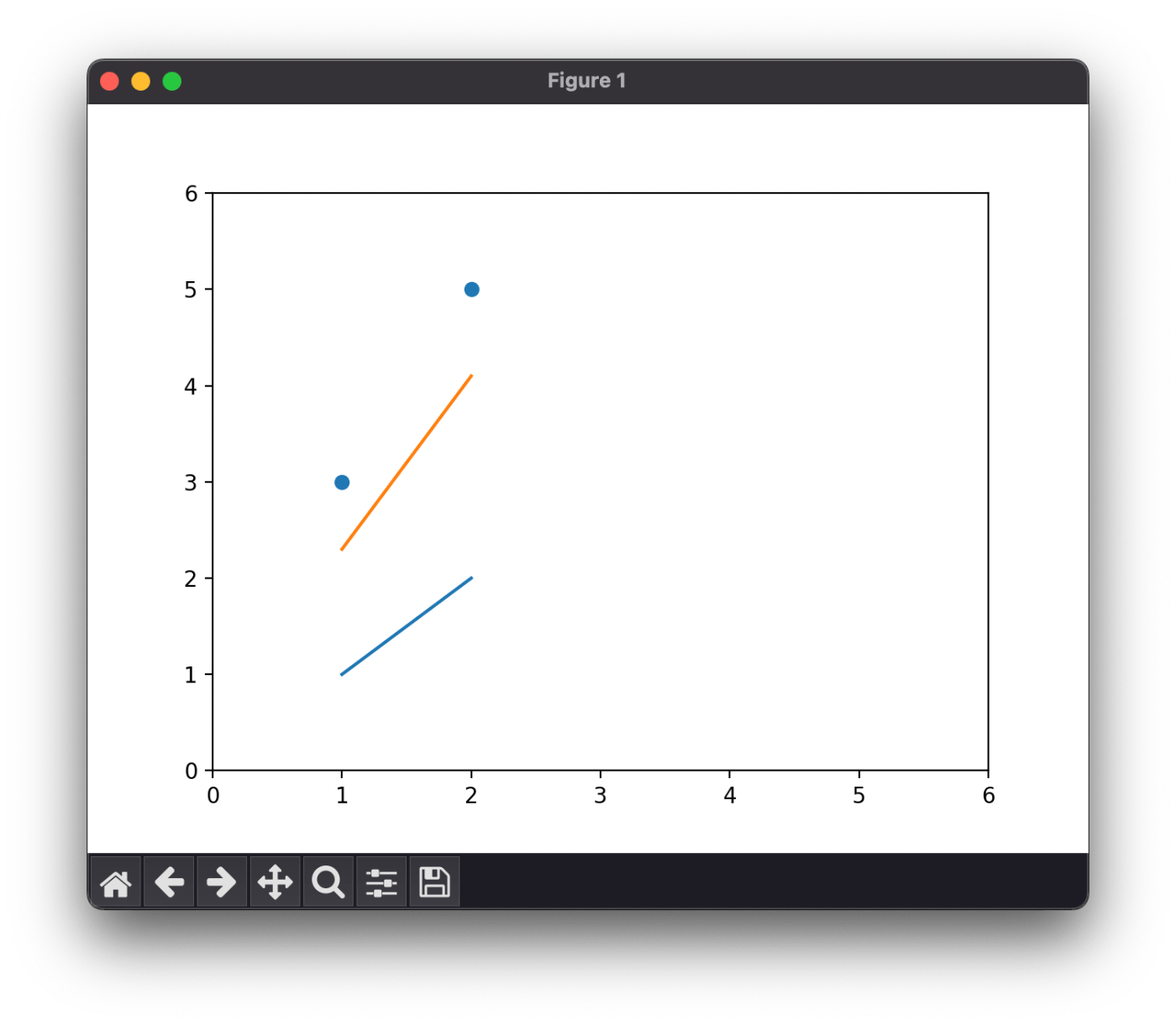
# 予測する
y = a * x + b
plt.plot(x, y.detach())
plt.show()
教師データは点、予測値は線でそれぞれ表示されている
勾配の算出
# 誤差との予測
e = torch.mean((t - y) ** 2)
e.backward();
print(a.grad, b.grad)
tensor(-8.) tensor(-5.)
となり、
一方、
偏微分値はこれらの平均を計算するようなので $\frac {\partial e} {\partial a} = (-4 - 12) / 2 = -8 となる。
一方 \frac {\partial e} {\partial b} = (-4 - 6) / 2 = 5$ となる。
学習
a = (a - a.grad * 0.1).detach().requires_grad_()
b = (b - b.grad * 0.1).detach().requires_grad_()
print(a, b)
print(a.grad, b.grad)
tensor(1.8000, requires_grad=True) tensor(0.5000, requires_grad=True)
None None
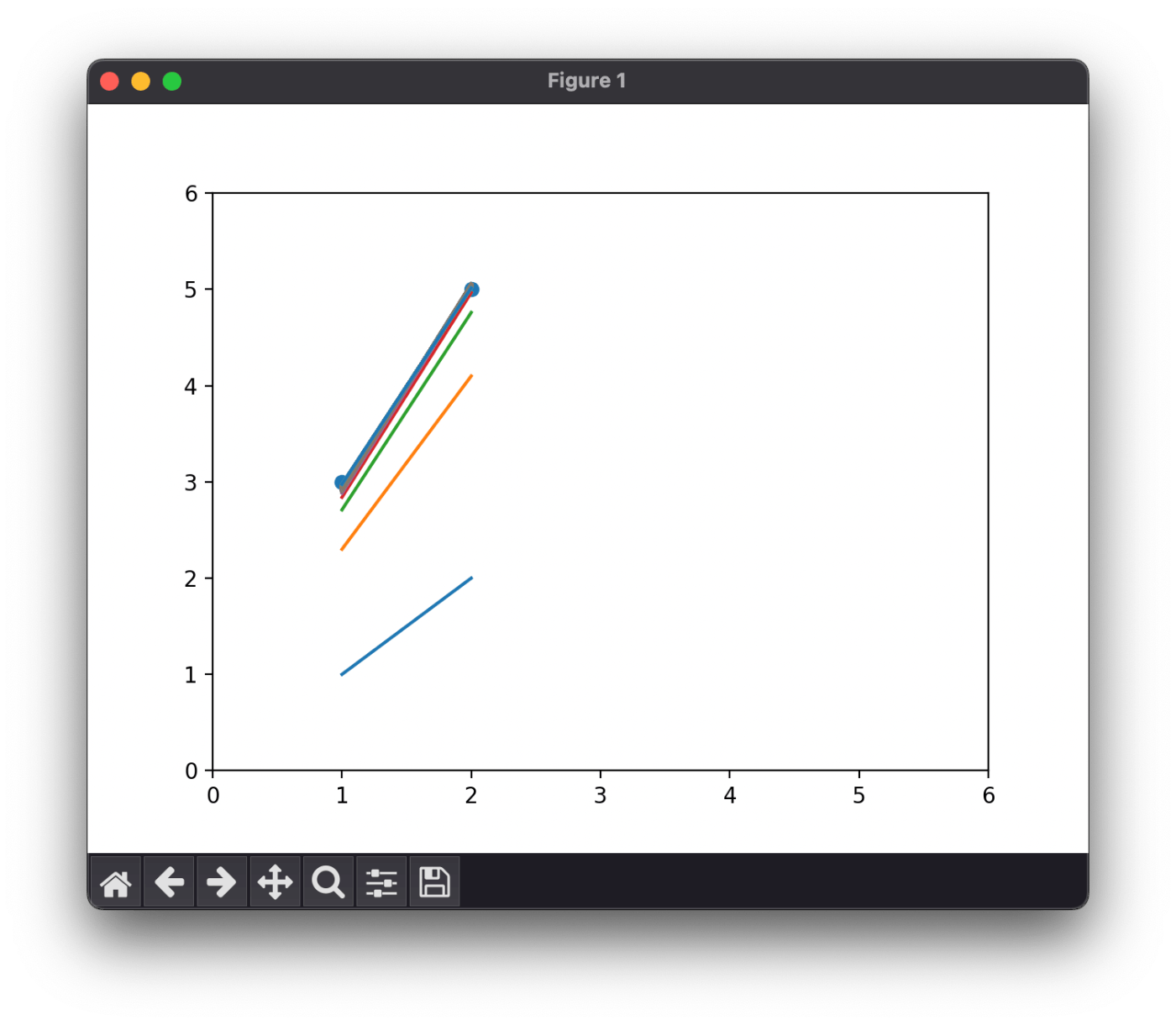
先ほどよりも教師データに近づいた
学習を 100 回繰り返す
# 学習の反復
for i in range(100):
    y = a * x + b
    plt.plot(x, y.detach())
    e = torch.mean((t - y) ** 2)
    e.backward()
    print(a.grad, b.grad)
    a = (a - a.grad * 0.1).detach().requires_grad_()
    b = (b - b.grad * 0.1).detach().requires_grad_()

print(a, b)
plt.show()
tensor(-2.5000) tensor(-1.6000)
tensor(-0.7700) tensor(-0.5300)
tensor(-0.2260) tensor(-0.1930)
...
tensor(0.0057) tensor(-0.0093)
tensor(2.0387, requires_grad=True) tensor(0.9374, requires_grad=True)
5/27 (土) はここまで
良い記事を見つけたおかげで loss.backward()、optimizer.step()、optimizer.zero_grad() が何をやっているのかをよく理解することができた。
昨日と今日、合わせて 1.5 時間くらいなので累計で 8.5 時間くらい。
そろそろ物体検出をやってみたい。
5/27 (土) おかわり
だいぶ寄り道してしまったが Quickstart に戻ろう。
評価の前に
# 評価します。
size = len(test_dataloader.dataset)
num_batches = len(test_dataloader)
print(size, num_batches)
10000 157
おそらくバッチサイズが 64 だから 10000 / 64 で 157 なのだろう。
評価
model.eval()
test_loss, correct = 0, 0
with torch.no_grad():
    for X, y in test_dataloader:
        X, y = X.to(device), y.to(device)
        pred = model(X)
        test_loss += loss_fn(pred, y).item()
        correct += (pred.argmax(1) == y).type(torch.float).sum().item()
test_loss /= num_batches
correct /= size
print(
    f"Test Error: \n Accuracy: {(100*correct):>0.1f}%, Avg loss: {test_loss:>8f} \n")
Test Error:
 Accuracy: 42.2%, Avg loss: 2.154667
最後に Jupyter の VSCode 拡張を試す
インストールしたら Command + Shift + P ">Create: New Jupyter Notebook" で Jupyter Notebook を作成する。
VSCode なんでもできるな。
コードの実行
▷ ボタンを押すか Ctrl + Enter で実行できる。
コードを追加するときは Esc + Command + Enter で良さそう。
VSCode の Jupyter 拡張が超絶楽ちん
なんで今まで使わなかったんだろうと思うレベル。
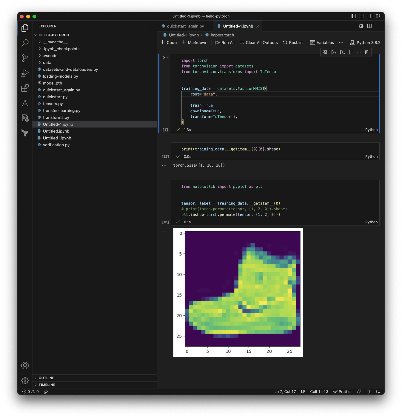
画像の表示までできる
気まぐれにやってみて良かった。
おわりに
最後は 30 分くらいだったので累計で 9 時間くらいを学習に費やした。
短くない時間ではあったがそれに見合う価値は合ったので満足している。
機械学習の勉強はこれまでサボってきたので世間一般のレベルに追いつくまでは大変だと思うがやっていて楽しく得るものも大きいので学習を続けたい。