状態空間モデル 論文解説⑤「 Mamba-2 」

論文

前回 は Mamba を解説しました。今回はその正当進化モデルである Mamba-2 です。

タイトル

Transformers are SSMs: Generalized Models and Efficient Algorithms Through Structured State Space Duality

論文: https://arxiv.org/pdf/2405.21060
Github: https://github.com/state-spaces/mamba

解説ステップ

概要

• 行列Aを対角からスカラーに変更した
• それ（とSSD※後述※）によりメモリ効率化を実現し、内部状態次元数が拡張された
• アーキテクチャーを一部変更し、Multi-head の概念を取り入れた
• 結果、性能アップとスピードアップを実現した

以上が、Mamba-2のモデルに対する概要になりますが、論文では多くの部分を以下について言及しています。

• Attention と SSM の比較
• SSD アルゴリズムの一般化

実は、SSDなどの高速計算部分などの理解を無視する場合、Mamba からの変更点は軽微です。しかし、その無視できる箇所が難解で、論文の理解を難しくしています。

本記事では、あくまで Mamba-2 のモデル構造に主眼を置きそれを軸に解説し、さらに後半で私が理解したところまでの「その他」の解説を試みます。

Mamba からの変更点

Mamba からのアップデートは、内部状態次元数を増やす 事が主眼だと思われます。なので、基本的な構造は似ています。

パラメータA(とD)をスカラーに変更

モデル構造 の章に詳細を書きますが、パラメータ$A$がスカラーになっています。

The structure on $𝐴$ is further simplified from diagonal to scalar times identity structure. Each $A_t$ can also be identified with just a scalar in this case.

※デフォルト設定では、パラメータ$D$もスカラーです。

Multi-head 化

パラメータ$A$,$D$ はヘッド単位で分かれ、$B$と$C$ はヘッドの渡って共通です。式で書くと以下になります。太字をベクトルもしくは行列として表しています。

$$\begin{align*} \underbrace{ \bold{h}_t^{(h)} }_{\in \mathbb{R}^{N \times P}} &= \underbrace{a_t^{(h)}}_{\in \mathbb{R}} \underbrace{ \bold{h}_{t-1}^{(h)} }_{\in \mathbb{R}^{N \times P}} + \underbrace{ \bold{B}_t }_{\in \mathbb{R}^{N \times 1}} \underbrace{ \bold{x}_{t}^{(h)} }_{\in \mathbb{R}^{1 \times P}} \\ \bold{y}_t^{(h)} &= \underbrace{ \bold{C}_t }_{\in \mathbb{R}^{1 \times N}} \bold{h}_t^{(h)} + \underbrace{d_t^{(h)}}_{\in \mathbb{R}} \bold{x}_{t}^{(h)} \\ \end{align*}$$

アーキテクチャーを変更

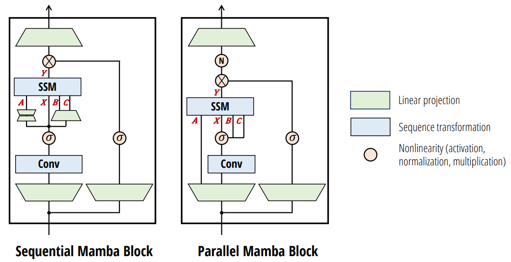
上図で、左：Mamba　右：Mamba-2 です。計算方法や、Aのパラメータの違いはありますが、構造レベルでいえばこれ以外は Mamba と同じです。

モデル構造 の章に詳細を書きます。

モデル構造

Pythonの簡易環境構築は前回資料を参考にしてください。

>>> model = MixerModel(128, 4, 128, 50277, ssm_cfg={"layer": "Mamba2", "d_ssm": 64, "headdim": 32})
>>> model
MixerModel(
  (embedding): Embedding(50277, 128)
  (layers): ModuleList(
    (0-3): 4 x Block(
      (norm): LayerNorm((128,), eps=1e-05, elementwise_affine=True)
      (mixer): Mamba2(
        (in_proj): Linear(in_features=128, out_features=770, bias=False)
        (conv1d): Conv1d(320, 320, kernel_size=(4,), stride=(1,), padding=(3,), groups=320)
        (act): SiLU()
        (norm): RMSNorm()
        (out_proj): Linear(in_features=256, out_features=128, bias=False)
      )
      (norm2): LayerNorm((128,), eps=1e-05, elementwise_affine=True)
      (mlp): GatedMLP(
        (fc1): Linear(in_features=128, out_features=256, bias=False)
        (fc2): Linear(in_features=128, out_features=128, bias=False)
      )
    )
  )
  (norm_f): LayerNorm((128,), eps=1e-05, elementwise_affine=True)
)

Mamba-2 Layer

コードを図に書き起こすと以下になります。

独自解釈が一部あります。B,Cで Group という Head とは違う概念が出てきます。これは head 横断でグループ共有（ngroups）しています。デフォルトでは ngroups=1 です。

B # バッチ数
T # 時系列長. sequence length
D # 入力次元. 言語モデルにおいてはトークンの embedding 次元
H    = 2      # Head の数
P    = 32     # 各 Head の次元数
N    = 128    # SSMの内部状態(h)の次元数
G    = 1      # B,Cのグループの数
Dssm = Nh x P # SSMに入力するxの次元数
Dmlp = 192    # Mamba Layer内部の MLP の次元数
Din  = Dssm + Dmlp
K    = 4      # 1次元畳み込みのカーネルサイズの初期値

各変数のshapeなど

>>> from mamba_ssm.modules.mamba2 import *
>>> self = model.layers[0].mixer
>>> self
Mamba2(
  (in_proj): Linear(in_features=128, out_features=770, bias=False)
  (conv1d): Conv1d(320, 320, kernel_size=(4,), stride=(1,), padding=(3,), groups=320)
  (act): SiLU()
  (norm): RMSNorm()
  (out_proj): Linear(in_features=256, out_features=128, bias=False)
)
>>> u = torch.rand(1, 16, 128)
>>> batch, seqlen, dim = u.shape
>>> conv_state, ssm_state = None, None
>>> zxbcdt = self.in_proj(u)  # (B, L, d_in_proj) or (B * L, d_in_proj)
>>> A = -torch.exp(self.A_log.float())  # (nheads) or (d_inner, d_state)
>>> d_mlp = (zxbcdt.shape[-1] - 2 * self.d_ssm - 2 * self.ngroups * self.d_state - self.nheads) // 2
>>> z0, x0, z, xBC, dt = torch.split(
    zxbcdt,
    [d_mlp, d_mlp, self.d_ssm, self.d_ssm + 2 * self.ngroups * self.d_state, self.nheads],
    dim=-1
)
>>> for x in [z0, x0, z, xBC, dt]: print(x.shape)
torch.Size([1, 16, 192])
torch.Size([1, 16, 192])
torch.Size([1, 16, 64])
torch.Size([1, 16, 320])
torch.Size([1, 16, 2])
>>> self.conv1d(xBC.transpose(1, 2)).shape
torch.Size([1, 320, 19])
>>> self.conv1d(xBC.transpose(1, 2)).transpose(1, 2).shape
torch.Size([1, 19, 320])
>>> xBC = self.act(
    self.conv1d(xBC.transpose(1, 2)).transpose(1, 2)[:, :-(self.d_conv - 1)]
)
>>> xBC.shape
torch.Size([1, 16, 320])
>>> x, B, C = torch.split(xBC, [self.d_ssm, self.ngroups * self.d_state, self.ngroups * self.d_state], dim=-1)
>>> for x in [x, B, C]: print(x.shape)
torch.Size([1, 16, 64])
torch.Size([1, 16, 128])
torch.Size([1, 16, 128])
>>> dt = F.softplus(dt + self.dt_bias.to(dtype=dt.dtype))
>>> dA = torch.exp(dt * A)
>>> x = rearrange(x, "b l (h p) -> b l h p", p=self.headdim)
>>> dB = torch.einsum("blh,bln->blhn", dt, B)
>>> dBx = torch.einsum("blhn,blhp->blhpn", dB, x)
>>> ssm_state = torch.rand(dBx.shape)
>>> ssm_state = ssm_state * rearrange(dA, "b l h -> b l h 1 1") + dBx
>>> ssm_state.shape
torch.Size([1, 16, 2, 32, 128])
>>> y = torch.einsum("blhpn,bln->blhp", ssm_state.to(dtype), C)
>>> y = y + rearrange(self.D.to(dtype), "h -> h 1") * x

補足① SSD アルゴリズム

敢えて、補足と書きます。Mamba の Selective Scan もそうですが、これらは計算とメモリ効率化の話であり、モデル構造そのものの本質ではないからです。

論文では当然重要と捉えていますが、あえて本記事では、このスタンスで解説を進めたいと思います。

SSM を行列Mで書き直す

SSMは次のように書けます。

$$\begin{align*} h_0 &= B_0 x_0 \\ y_0 &= C_0^T B_0 x_0 \\ h_1 &= A_1 h_0 + B_1 x_1 = A_1 B_0 x_0 + B_1 x_1 \\ y_1 &= C_1^T A_1 B_0 x_0 + C_1^T B_1 x_1 \\ h_2 &= A_2 h_1 + B_2 x_2 = A_2 A_1 B_0 x_0 + A_2 B_1 x_1 + B_2 x_2 \\ y_2 &= C_2^T A_2 A_1 B_0 x_0 + C_2^T A_2 B_1 x_1 + C_2^T B_2 x_2 \\ h_3 &= A_3 h_2 + B_3 x_3 = A_3 A_2 A_1 B_0 x_0 + A_3 A_2 B_1 x_1 + A_3 B_2 x_2 + B_3 x_3 \\ y_3 &= C_3^T A_2 A_1 B_0 x_0 + C_3^T A_3 A_2 B_1 x_1 + C_3^T A_3 B_2 x_2 + C_3^T B_3 x_3 \\ ... \end{align*}$$

これを一般化すると以下のようになります。

$$\begin{bmatrix} y_0 \\ y_1 \\ y_2 \\ y_3 \\ \vdots \\ \vdots \\ \vdots \\ y_j \\ \end{bmatrix}= \begin{bmatrix} C_0^T B_0 & & & & & & & \\ C_1^T A_1 B_0 & C_1^T B_1 & & & & & & \\ C_2^T A_2 A_1 B_0 & C_2^T A_2 B_1 & C_2^T B_2 & & & & & \\ C_3^T A_3 A_2 A_1 B_0 & C_3^T A_3 A_2 B_1 & C_3^T A_3 B_2 & C_3^T B_3 & & & & \\ \vdots & \vdots & \vdots & \vdots & \ddots & & & \\ \vdots & \vdots & \vdots & \vdots & & \ddots & & \\ \vdots & \vdots & \vdots & \vdots & & & \ddots & \\ C_j^T A_j A_{j-1} ... A_1 B_0 & C_j^T A_j A_{j-1} ... A_2 B_1 & C_j^T A_j A_{j-1} ... A_3 B_2 & C_j^T A_j A_{j-1} ... A_4 B_3 & \cdots & C_j^T A_j ... A_{i+1} B_i & \cdots & C_j^T B_j \\ \end{bmatrix} \begin{bmatrix} x_0 \\ x_1 \\ x_2 \\ x_3 \\ \vdots \\ \vdots \\ \vdots \\ x_j \\ \end{bmatrix}$$

つまり以下のように一般化できます。

$$\bold{y}=SSM(\bold{A},\bold{B},\bold{C})(\bold{x})=\bold{M} \bold{x}$$

N-SSS (N-sequentially semiseparable) 行列

上述の行列$M$は各変数が次のような次元Nを持つ場合、N-SSS 行列と呼びます。

$$\begin{align*} \bold{A}&=(A_0, ..., A_i, ..., A_{T-1}), A_i \in \mathbb{R}^{N \times N} \\ \bold{B}&=(B_0, ..., B_i, ..., B_{T-1}), B_i \in \mathbb{R}^{N} \\ \bold{C}&=(C_0, ..., C_i, ..., C_{T-1}), C_i \in \mathbb{R}^{N} \\ \end{align*}$$

要素別にまとめると以下です。

$$M_{ji}= \begin{dcases} C_j^T B_j & j=i, \\ C_j^T(A_{j} A_{j-1} ... A_{i+1}) B_i & j>i, \\ 0 & j<i, \\ \end{dcases}$$

N-semiseparable 行列 ※本記事ではほとんど関係ありません

次のようなベクトル列とスカラー$d_i \in \mathbb{R} \ \ \ \ \ (i=1, ..., L)$があります。

$$p_i, q_i, r_i, s_i \in \mathbb{R}^{N} \ \ \ \ \ (i=1, ..., L) \\$$

これらを使って以下のように行列Sが書けるとします。

$$S=\begin{bmatrix} d_1 & r_1^T s_2 & r_1^T s_3 & \cdots & r_1^T s_T \\ p_2^T q_1 & d_2 & r_2^T s_3 & \cdots & r_2^T s_T \\ p_3^T q_1 & p_3^T q_2 & d_3 & \cdots & r_3^T s_T \\ \vdots & \vdots & \vdots & \ddots & \vdots \\ p_T^T q_1 & p_T^T q_2 & p_T^T q_3 & \cdots & d_T \\ \end{bmatrix}$$

するとこの行列Sは次のように分解でき、簡略化できます。

$$S=diag(d) + tril(\bold{P} \bold{Q}^⊤,−1) + triu(\bold{R} \bold{S}^⊤,1)$$

※tril や triu は下三角、上三角へのマスク処理です。

N-SSS の一般系

N-SSのさらに特殊な形を表します。次のような

スカラー列

$$d_i \in \mathbb{R} \ \ \ \ \ (i=1, ..., T)$$

ベクトル列

$$p_i, q_i, r_i, s_i \in \mathbb{R}^{N} \ \ \ \ \ (i=1, ..., T) \\$$

行列　列

$$\Phi_i, \Psi_i \in \mathbb{R}^{N\times N} \ \ \ \ \ (i=1, ..., T) \\$$

があります。これらを使って以下のように行列Sが書けるとします。

$$S=\begin{bmatrix} d_1 & r_1^T \Psi_2 s_2 & r_1^T \Psi_2 \Psi_3 s_3 & \cdots & r_1^T \Psi_2 ... \Psi_{T} s_T \\ p_2^T \Phi_2 q_1 & d_2 & r_2^T \Psi_3 s_3 & \cdots & r_2^T \Psi_3 ... \Psi_{T} s_T \\ p_3^T \Phi_3 \Phi_2 q_1 & p_3^T \Phi_3 q_2 & d_3 & \cdots & r_3^T \Psi_4 ... \Psi_{T} s_T \\ \vdots & \vdots & \vdots & \ddots & \vdots \\ p_T^T \Phi_{T} ... \Phi_2 q_1 & p_T^T \Phi_{T} ... \Phi_3 q_2 & p_T^T \Phi_{T} ... \Phi_4 q_3 & \cdots & d_T \\ \end{bmatrix}$$

これを要素別にまとめると以下のようになります。

$$S_{ij}= \begin{dcases} d_i & i=j, \\ p_i^T(\Phi_{i} \Phi_{i-1} ... \Phi_{j+1}) q_j & i>j, \\ r_i^T(\Psi_{i+1} \Psi_{i+2} ... \Psi_{j} ) s_j & i<j, \\ \end{dcases}$$

1-SS 行列

まず、1-SSS を記述してみましょう。$N=1$、つまり各時系列点にある変数が全てスカラーになります。スカラーなので、全て小文字で表してみます。

$$\begin{bmatrix} c_0 b_0 & & & & & & \\ c_1 a_1 b_0 & c_1 b_1 & & & & & \\ c_2 a_2 a_1 b_0 & c_2 a_2 b_1 & c_2 b_2 & & & & \\ \vdots & \vdots & \vdots & \ddots & & & \\ & & & & \ddots & & \\ & & & c_j a_j a_{j-1} ... a_{i+1} b_i & & \ddots & \\ & & & & & & c_{T-1} b_{T-1} \\ \end{bmatrix}$$

これをさらに分解すると、次のようになります。

$$\bold{y}= \begin{bmatrix} c_0 & & & & & & \\ & c_1 & & & & & \\ & & c_2 & & & & \\ & & & \ddots & & & \\ & & & & & & \\ & & & & & & \\ & & & & & & c_{T-1}\\ \end{bmatrix} \underbrace{ \begin{bmatrix} 1 & & & & & & \\ a_1 & 1 & & & & & \\ a_2 a_1 & a_2 & 1 & & & & \\ \vdots & \vdots & \vdots & \ddots & & & \\ & & & & \ddots & & \\ & & & a_j a_{j-1} ... a_{i+1} & & \ddots & \\ & & & \cdots & & & 1 \\ \end{bmatrix} }_{L: 1-SS} \begin{bmatrix} b_0 & & & & & & \\ & b_1 & & & & & \\ & & b_2 & & & & \\ & & & \ddots & & & \\ & & & & & & \\ & & & & & & \\ & & & & & & b_{T-1}\\ \end{bmatrix} \bold{x}$$

この真ん中の $a$ で構成された行列を、1-SS 行列（$L$と置きます）と定義します。実はこのようにスカラーにすることで、以下のような式変形が可能になります。

$$\bold{y}=\underbrace{L}_{\in \mathbb{R}^{T \times T}} \odot (\underbrace{C}_{\in \mathbb{R}^{T \times 1}}\underbrace{B^T}_{\in \mathbb{R}^{1 \times T}})\underbrace{\bold{x}}_{\in \mathbb{R}^{T \times P}}$$

これはスカラーになる事で計算を単純化している、と言いたい訳ではありません。実際に効率化された計算はこれらをさらにチャンクに分けて、並列計算により計算を効率化しています。
この形式の表現は、1-SS（下三角の半可分）に落とすと Structured Masked Attention の形に一致する 事が重要であり、Attention との比較が明確になります。

N-SSSをチャンクに分けて構造化

さて、Mamba の Selective Scan にあたる箇所を、より高速化した計算方法を解説します。行列$\bold{M}$と入力$\bold{x}$ある適当なサイズでチャンクに分割する事を考えます。

実はチャンクに分ける事で、$M=L \odot CB^T$ を直接計算するより計算量を減らせるのです。

実際のSSDはN-SSS(N=1)を想定していますが、以下の解説ではランクNのままで一般化された形式で表記します。

この N-SSS 行列は適当なチャンクに分割した際、さらに同じような構造が現れます。上図ではチャンクサイズ$Q=3$で区切っており、色が分かれている箇所を次のようなブロック名で定義します。

上図の左側は、計算結果を連続している絵ですが、これは疑似コードの解説まで触れた時に理解できるかと思います。

さて、行列$M \in \mathbb{R}^{T \times T}$をチャンクサイズ$Q$で区切って$M'$を定義します。

$$M'= \begin{bmatrix} M^{(0,0)} & & & & \\ M^{(1,0)} & M^{(1,1)} & & & \\ M^{(2,0)} & M^{(2,1)} & M^{(2,2)} & & \\ \vdots & \vdots & \vdots & \ddots & \\ M^{(T/Q-1,0)} & M^{(T/Q-1,1)} & M^{(T/Q-1,2)} & \cdots & M^{(T/Q-1,T/Q-1)} \\ \end{bmatrix}$$

この時、対角成分は以下のようになります。

$$M^{(j,j)}=O_j=SSM(A_{jQ:(j+1)Q}, B_{jQ:(j+1)Q}, C_{jQ:(j+1)Q})$$

それ以外の成分（$S$: Left, $U$: Center, $R$: Right）は以下です。

$$M^{(j,i)}=S_j U_{j:i} R_i= \begin{bmatrix} C_{jQ}^T A_{jQ:jQ-1} \\ \vdots \\ C_{(j+1)Q-1}^T A_{(j+1)Q-1:jQ-1} \\ \end{bmatrix} A_{jQ-1:(i+1)Q-1} \begin{bmatrix} B_{iQ}^T A_{(i+1)Q-1:iQ} \\ \vdots \\ B_{(i+1)Q-1}^T A_{(i+1)Q-1:(i+1)Q-1} \\ \end{bmatrix}^T$$

$S$ は $j$ のみで決まり、つまり行列の縦の値は全て同じで、$R$ は $i$ のみで決まり、つまり行列の横の値は全て同じになります。$U_i$ を次のように定義します。

$$\begin{align*} U_{j:j-1} &= A_{jQ-1:jQ-1} = 1 \\ U_{j:j-2} &= A_{jQ-1:(j-1)Q-1} \colonequals U_j \\ U_{j:j-3} &= A_{jQ-1:(j-2)Q-1}=A_{jQ-1:(j-1)Q-1} A_{(j-1)Q-1:(j-2)Q-1}=U_j U_{j-1} \\ \cdots & \\ U_{j:i} &= U_j U_{j-1} ... U_{i+2} \end{align*}$$

大文字で書いていますが、SSDにおいては全てスカラーです。あくまで一般的な形式で書いています。

さて、改めて$O$,$S$,$U$,$R$ で $M'$ を書き直します。

$$M'= \begin{bmatrix} O_0 & & & & \\ S_1 U_{1:0} R_0 & O_1 & & & \\ S_2 U_{2:0} R_0 & S_2 U_{2:1} R_1 & O_2 & & \\ S_3 U_{3:0} R_0 & S_3 U_{3:1} R_1 & S_3 U_{3:2} R_2 & & \\ \vdots & \vdots & \vdots & \ddots & \\ S_{T/Q-1} U_{T/Q-1:0} R_0 & S_{T/Q-1} U_{T/Q-1:1} R_1 & S_{T/Q-1} U_{T/Q-1:2} R_2 & \cdots & O_{T/Q-1} \\ \end{bmatrix}$$

$$=\begin{bmatrix} O_0 & & & & \\ S_1 R_0 & O_1 & & & \\ S_2 U_2 R_0 & S_2R_1 & O_2 & & \\ S_3 U_3 U_2 R_0 & S_3 U_3 R_1 & S_3 R_2 & & \\ \vdots & \vdots & \vdots & \ddots & \\ S_{T/Q-1} U_{T/Q-1} ... U_2 R_0 & S_{T/Q-1} U_{T/Q-1} ... U_3 R_1 & S_{T/Q-1} U_{T/Q-1} ... U_4 R_2 & \cdots & O_{T/Q-1} \\ \end{bmatrix}$$

するとどうでしょう。再度、N-SSS 行列が現れました。このように、N-SSSは別のN-SSSの構造で書き表すことができます。

同様に $\bold{x}$ をチャンクサイズ$Q$ で区切ったものを $\bold{X}=(X_0, ..., X_{T/Q-1})$とします。

$$M'X= diag(S_0, ... ,S_{T/Q-1}) \begin{bmatrix} 0 & & & & & \\ I & 0 & & & & \\ U_2 & I & 0 & & & \\ U_3 U_2 & U_3 & I & \ddots & & \\ \vdots & & & \ddots & 0 & \\ U_{T/Q-1} ... U_2 & \cdots & & & I & 0\\ \end{bmatrix} diag(R_0, ... ,R_{T/Q-1}) \bold{X} + diag(O)\bold{X}$$

こちらをさらに整理すると

$$=\underbrace{ diag(S_0, ... ,S_{T/Q-1}) }_{T/Q \times T/Q \times ( Q \times H )} \underbrace{ \begin{bmatrix} 0 & & & & & \\ I & 0 & & & & \\ U_2 & I & 0 & & & \\ U_3 U_2 & U_3 & I & \ddots & & \\ \vdots & & & \ddots & 0 & \\ U_{T/Q-1} ... U_2 & \cdots & & & I & 0\\ \end{bmatrix} }_{T/Q \times T/Q \times ( H \times H )} \underbrace{ \begin{bmatrix} R_0 X_0 \\ R_1 X_1 \\ R_2 X_2 \\ R_3 X_3 \\ \vdots \\ R_{T/Q-1} X_{T/Q-1} \\ \end{bmatrix} }_{T/Q \times (H \times Q) \times (Q \times P)} + \underbrace{ \begin{bmatrix} O_0 X_0 \\ O_1 X_1 \\ O_2 X_2 \\ O_3 X_3 \\ \vdots \\ O_{T/Q-1} X_{T/Q-1} \\ \end{bmatrix} }_{T/Q \times SSM(Q \times P)}$$

Mamba と同様、この構造を並列化を駆使して計算します。

SSDの具体的な計算

以下は「Listing 1 Full PyTorch example of the state space dual (SSD) model」の疑似コードをそのまま使えるように少し修正したプログラムです。

import torch 
from einops import rearrange
import torch.nn.functional as F

def segsum(x):
    """Naive segment sum calculation. exp(segsum(A)) produces a 1-SS matrix,
    which is equivalent to a scalar SSM."""
    T = x.size(-1)
    x_cumsum = torch.cumsum(x, dim=-1)
    x_segsum = x_cumsum[..., :, None] - x_cumsum[..., None, :]
    mask = torch.tril(torch.ones(T, T, device=x.device, dtype=bool), diagonal=0)
    x_segsum = x_segsum.masked_fill(~mask, -torch.inf)
    return x_segsum

def ssd(X, A, B, C, block_len=64, initial_states=None):
    """
    Arguments:
    X: (batch, length, n_heads, d_head)
    A: (batch, length, n_heads)
    B: (batch, length, n_heads, d_state)
    C: (batch, length, n_heads, d_state)
    Return:
    Y: (batch, length, n_heads, d_head)
    """
    assert X.dtype == A.dtype == B.dtype == C.dtype
    assert X.shape[1] % block_len == 0
    # Rearrange into blocks/chunks
    X, A, B, C = [rearrange(x, "b (c l) ... -> b c l ...", l=block_len) for x in (X, A, B, C)]
    A = rearrange(A, "b c l h -> b h c l") # b: B, h: H, c: T/Q, l: Q
    A_cumsum = torch.cumsum(A, dim=-1)
    # 1. Compute the output for each intra-chunk (diagonal blocks)
    L = torch.exp(segsum(A))
    Y_diag = torch.einsum("bclhn,bcshn,bhcls,bcshp->bclhp", C, B, L, X) # n: N, s: Q, p: P
    # 2. Compute the state for each intra-chunk
    # (right term of low-rank factorization of off-diagonal blocks; B terms)
    decay_states = torch.exp((A_cumsum[:, :, :, -1:] - A_cumsum))
    states = torch.einsum("bclhn,bhcl,bclhp->bchpn", B, decay_states, X)
    # 3. Compute the inter-chunk SSM recurrence; produces correct SSM states at chunk boundaries
    # (middle term of factorization of off-diag blocks; A terms)
    if initial_states is None:
        initial_states = torch.zeros_like(states[:, :1])
    states = torch.cat([initial_states, states], dim=1)
    decay_chunk = torch.exp(segsum(F.pad(A_cumsum[:, :, :, -1], (1, 0))))
    new_states = torch.einsum("bhzc,bchpn->bzhpn", decay_chunk, states)
    states, final_state = new_states[:, :-1], new_states[:, -1]
    # 4. Compute state -> output conversion per chunk
    # (left term of low-rank factorization of off-diagonal blocks; C terms)
    state_decay_out = torch.exp(A_cumsum)
    Y_off = torch.einsum('bclhn,bchpn,bhcl->bclhp', C, states, state_decay_out)
    # Add output of intra-chunk and inter-chunk terms (diagonal and off-diagonal blocks)
    Y = rearrange(Y_diag+Y_off, "b c l h p -> b (c l) h p")
    return Y, final_state

if __name__ == "__main__":
    batch     = 2                  # B
    length    = 72                 # T
    n_heads   = 4                  # H
    dim_din   = 512                # Din
    d_head    = dim_din // n_heads # P
    d_state   = 32                 # N
    block_len = 8                  # Q
    X = torch.randn(batch, length, n_heads, d_head)
    A = -F.softplus(torch.randn(batch, length, n_heads))
    B = torch.randn(batch, length, n_heads, d_state)
    C = torch.randn(batch, length, n_heads, d_state)
    Y, final_state = ssd(X, A, B, C, block_len=block_len)
    print(Y.shape)
    print(final_state.shape)

segsum は次のような操作になります。

>>> segsum(torch.arange(1, 5, dtype=float).reshape(1, 1, -1))
tensor([[[[0., -inf, -inf, -inf],
          [2., 0., -inf, -inf],
          [5., 3., 0., -inf],
          [9., 7., 4., 0.]]]], dtype=torch.float64)

これは次のようなマトリクスを作っています。（$X=(X_0, X_1, X_2, X_3)$）

$$Y=segsum(X)= \begin{bmatrix} 0 & -inf & -inf & -inf \\ X_1 & 0 & -inf & -inf \\ X_2 + X_1 & X_2 & 0 & -inf \\ X_3 + X_2 + X_1 & X_3 + X_2 & X_3 & 0 \\ \end{bmatrix}$$

そしてこれを以下のように exp を操作する事で、1-SS行列を作成します。($A_i = exp(X_i)$)

$$L=exp(Y)= \begin{bmatrix} 1 & 0 & 0 & 0 \\ A_1 & 1 & 0 & 0 \\ A_2 A_1 & A_2 & 1 & 0 \\ A_3 A_2 A_1 & A_3 A_2 & A_3 & 1 \\ \end{bmatrix}$$

X, A, B, C = [rearrange(x, "b (c l) ... -> b c l ...", l=block_len) for x in (X, A, B, C)]
A = rearrange(A, "b c l h -> b h c l")
L = torch.exp(segsum(A))
Y_diag = torch.einsum("bclhn,bcshn,bhcls,bcshp->bclhp", C, B, L, X)

これは $O_i X_i$ を計算しています。

Y = A_cumsum[:, :, :, -1:] - A_cumsum の操作は

$$\begin{align*} A_{cumsum} &= (X_0, X_0 + X_1, X_0 + X_1 + X_2, X_0 + X_1 + X_2 + X_3) \\ Y &= (X_0 + X_1 + X_2 + X_3 - (X_0), ..., X_0 + X_1 + X_2 + X_3 - (X_0 + X_1 + X_2 + X_3)) \\ &= (X_3 + X_2 + X_1, X_3 + X_2, X_3, 0) \\ \end{align*}$$

となり、よって

>>> decay_states = torch.exp((A_cumsum[:, :, :, -1:] - A_cumsum))
>>> states = torch.einsum("bclhn,bhcl,bclhp->bchpn", B, decay_states, X)
>>> states.shape
torch.Size([2, 9, 4, 128, 32])

この操作は $R_i X_i$ を計算しています。

A_cumsum[:, :, :, -1] について考えてみます。これは、各チャンクの最終配列です。batch と head 次元を無視すると、$A=(A_0, ..., A_8)$ で $Q=3$ とすれば、それをチャンクに分ける事で $A$ と $A_{cumsum}$ は以下のようになります。

$$A=\begin{bmatrix} A_0 & A_1 & A_2 \\ A_3 & A_4 & A_5 \\ A_6 & A_7 & A_8 \\ \end{bmatrix}, A_{cumsum}=\begin{bmatrix} A_0 & A_1 + A_0 & A_2 + A_1 + A_0 \\ A_3 & A_4 + A_3 & A_5 + A_4 + A_3 \\ A_6 & A_7 + A_6 & A_8 + A_7 + A_6 \\ \end{bmatrix}$$

つまり、Y=F.pad(A_cumsum[:, :, :, -1], (1, 0)) は

$$Y=\begin{bmatrix} 0 & A_2 + A_1 + A_0 & A_5 + A_4 + A_3 & A_8 + A_7 + A_6 & \end{bmatrix}$$

プログラムで書いてみると以下です。

>>> A = torch.arange(1, 10).to(float).reshape(-1, 3)
>>> A
tensor([[1., 2., 3.],
        [4., 5., 6.],
        [7., 8., 9.]], dtype=torch.float64)
>>> A_cumsum
tensor([[ 1.,  3.,  6.],
        [ 4.,  9., 15.],
        [ 7., 15., 24.]], dtype=torch.float64)
>>> F.pad(A_cumsum[:, -1], (1, 0))
tensor([ 0.,  6., 15., 24.], dtype=torch.float64)
>>> segsum(F.pad(A_cumsum[:, -1], (1, 0)))
tensor([[ 0., -inf, -inf, -inf],
        [ 6.,  0., -inf, -inf],
        [21., 15.,  0., -inf],
        [45., 39., 24.,  0.]], dtype=torch.float64)

です。もうお分かりかと思いますが、

>>> decay_chunk = torch.exp(segsum(F.pad(A_cumsum[:, :, :, -1], (1, 0))))

この操作は、Center Factor x Right Factor を表します。そのまま Left の流れも同様です。以上が、SSDの操作です。

このように、N-SSS の中に N-SSS が現れる事を利用して、Qのサイズでチャンク化する事で、計算量を減らせる仕組みとなっています。

疑問点

ただ、上記の計算ですが、少し間違っているかもしれません。というのも Center Factor で

$$U_{j:i}=A_{jQ-1:(i+1)Q-1}$$

となっている以上、例えば $Q=3$ の時に、$A_2 A_1 A_0$ という組は現れるはずがありません。なぜなら、$i=0$ のとき $U_{j:0}=A_{3j-1:2}$ となるからです。しかしながら疑似コードでは $A_2 + A_1 + A_0$の計算も使用されており、少しよく分かりません。

私の式展開か疑似コードのどこかが間違っている可能性があります。ただ、ここでは計算の雰囲気がつかめれば問題ないとも思っています。

補足② SSMとAttention の比較

こちらも敢えて、補足と書きます。論文では当然重要な内容となっていますが、Mamba-2 の構造を単に理解するだけなら、避けて通れる内容にはなります。

申し訳ありませんが、こちらは機会があれば解説を試みたいと思います。これまで解説でだいぶ体力を使ってしまいました...。