Numpy で時系列データに Rolling 処理を行う
Pandas の rolling メソッドと同じような処理を Numpy でも実現できないか、というのを調べたので、まとめます。
結論からいえば、Numpy.lib.stride_tricks.sliding_window_view 関数を用いるのが簡単そうでした。
Numpy による Rolling 処理の調査
Google 検索で、Numpy rolling で調べてみると、
- Numpy.roll()
- Numpy.lib.stride_tricks.as_strided()
を用いる方法などがひっかかりました。
Numpy.roll() はデータを環状にして、特定の軸方向に回転させるような処理で、データの開始点をずらすときに用いられるようです。
ですので、今回の目的には合いません。
次に、Numpy.lib.stride_tricks.as_strided() ですが、こちらはこの記事で紹介されているとおり、Pandas の rolling メソッドと同じ処理ができるようです。
しかしながら、窓のスライド幅(ストライド数)を Byte で指定する必要があり、使いやすくはなさそうです。
一方で、今回ご紹介する Numpy.lib.stride_tricks.sliding_window_view() は、窓の shape と窓をスライドさせる軸を指定するだけで Pandas の rolling () とほぼ同じ処理が可能です。
こちらの関数は、2021年1月30日にリリースされた Numpy 1.20.0 で追加されましたので、比較的新しい関数になります。
そのためなのか、あまり sliding_window_view() を取り上げた記事が見当たりませんでした。
sliding_window_view() で rolling 処理
時系列処理における例を3つ載せます。
1次元配列に区間数3の窓をスライドさせた場合
In [1]: import numpy as np

In [2]: from numpy.lib.stride_tricks import sliding_window_view

In [3]: x = np.arange(10)

In [4]: x
Out[4]: array([0, 1, 2, 3, 4, 5, 6, 7, 8, 9])

In [5]: sliding_window_view(x, 3)
Out[5]:
array([[0, 1, 2],
       [1, 2, 3],
       [2, 3, 4],
       [3, 4, 5],
       [4, 5, 6],
       [5, 6, 7],
       [6, 7, 8],
       [7, 8, 9]])
2次元配列に区間数3の窓を行方向(0軸方向)にスライドさせた場合
In [6]: x = np.arange(10).reshape(5, 2)

In [7]: x
Out[7]:
array([[0, 1],
       [2, 3],
       [4, 5],
       [6, 7],
       [8, 9]])

In [8]: sliding_window_view(x, 3, axis=0)
Out[8]:
array([[[0, 2, 4],
        [1, 3, 5]],

       [[2, 4, 6],
        [3, 5, 7]],

       [[4, 6, 8],
        [5, 7, 9]]])
2次元配列に次数3の移動平均を行方向に適用する場合
In [9]: x
Out[9]:
array([[0, 1],
       [2, 3],
       [4, 5],
       [6, 7],
       [8, 9]])

In [10]: sliding_window_view(x, 3, axis=0).mean(axis=-1)
Out[10]:
array([[2., 3.],
       [4., 5.],
       [6., 7.]])
最後に
公式ドキュメントには注意書きとして、以下の記述があります。
For many applications using a sliding window view can be convenient, but potentially very slow. Often specialized solutions exist, for example:
scipy.signal.fftconvolve
filtering functions in scipy.ndimage
moving window functions provided by bottleneck.
As a rough estimate, a sliding window approach with an input size of N and a window size of W will scale as O(N*W) where frequently a special algorithm can achieve O(N). That means that the sliding window variant for a window size of 100 can be a 100 times slower than a more specialized version.
Nevertheless, for small window sizes, when no custom algorithm exists, or as a prototyping and developing tool, this function can be a good solution.
sliding_window_axis() は便利な一方で、移動平均のような特別なケースに対応した関数と比べると処理が遅くなるそうです。
他に解決策がないときに最終手段としてこの関数を用いるのが良さそうですね。
ちなみに、私は itertools.groupby と併用して、グループごとに rolling 処理を実施しています。
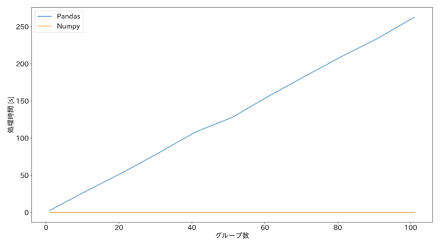
Pandas では、Groupby.rolling.apply() がありますが、こちらはグループ数が多くなるにつれてめちゃくちゃ処理時間が遅くなるのが、実験的にわかりました。
以下のグラフは、グループ数に対する処理時間(移動平均)を Pandas で処理した場合の
df.groupby(Groups).rolling(winsize).apply(lambda x: x.mean())
と、itertools.groupby() と sliding_window_axis() を用いた場合の
[moving_average(list(x), winsize) for _, x in it.groupby(df.to_numpy(), key=lambda x: x[0])]
で、処理速度を比較した結果です。
詳しい実験方法は省略しますが、Pandas で処理した場合はグループ数に比例して処理時間が大きくなっていくのに対して、itertools と Numpy を併用した場合は処理速度が大きく変わることはありませんでした。
実験に使用したコードは以下のとおりです。
import itertools as it
import os
import time

import japanize_matplotlib
import matplotlib as mpl
import matplotlib.pyplot as plt
import numpy as np
import pandas as pd
from tqdm import tqdm


def moving_average(x, winsize):
    x = np.array(x)[:, 1:].astype(np.float32)
    results = np.full(x.shape, np.nan)
    rolled = np.lib.stride_tricks.sliding_window_view(x, winsize, axis=0)
    results[winsize - 1 :] = rolled.mean(axis=2)
    return results


np.random.seed(1234)
mpl.rcParams["font.size"] = 18
japanize_matplotlib.japanize()

# 設定
stride = 10
n_groups_list = np.arange(1, 100 + stride, stride)
nrows = 200
ncols = 50
winsize = 20

# データ準備
data_size = (n_groups_list[-1] * nrows, ncols)
groups = np.array(sorted(list(range(n_groups_list[-1])) * nrows)).reshape(-1, 1)
data = np.random.standard_normal(data_size)
base = pd.DataFrame(np.concatenate([groups.astype(int), data], axis=1))
base = base.rename(columns={0: "Groups"})

# 処理時間の計測
pandas_times = []
numpy_times = []
for i in tqdm(range(0, n_groups_list.size)):
    df = base.loc[base["Groups"].isin(list(range(n_groups_list[i])))]

    start = time.time()
    results_pandas = (
        df.groupby("Groups").rolling(winsize).apply(lambda x: x.mean()).drop(columns="Groups")
    )
    pandas_times += [time.time() - start]

    start = time.time()
    results_numpy = [
        moving_average(list(x), winsize) for _, x in it.groupby(df.to_numpy(), key=lambda x: x[0])
    ]
    results_numpy = pd.DataFrame(np.vstack(results_numpy), columns=np.arange(1, ncols + 1))
    results_numpy = pd.concat([df["Groups"].reset_index(drop=True), results_numpy], axis=1)
    numpy_times += [time.time() - start]

# データ数に対する処理時間の関係をグラフ化
fig, ax = plt.subplots(figsize=(16, 9))
ax.plot(n_groups_list, pandas_times, label="Pandas")
ax.plot(n_groups_list, numpy_times, label="Numpy")
ax.set(xlabel="グループ数", ylabel="処理時間 [s]")
ax.legend()
fig.tight_layout()

savename = "./groupby_rolling_apply/groups_vs_time.png"
os.makedirs(os.path.dirname(savename), exist_ok=True)
plt.savefig(savename, dpi=300)
plt.close()

# 計算結果のプロット
results_pandas = results_pandas.reset_index()

fig, ax = plt.subplots(figsize=(16, 9))
show_groups = [1]
data_1 = results_pandas.loc[results_pandas["Groups"].isin(show_groups), 1].to_numpy()
data_2 = results_numpy.loc[results_numpy["Groups"].isin(show_groups), 1].to_numpy()
ax.plot(np.arange(data_1.shape[0]), data_1, label="Pandas")
ax.plot(np.arange(data_1.shape[0]), data_2, ls="--", label="Numpy")
ax.set(xlabel=r"$x_t$", ylabel=r"$y_t$")
ax.legend()
fig.tight_layout()

savename = "./groupby_rolling_apply/time-series-plot.png"
os.makedirs(os.path.dirname(savename), exist_ok=True)
plt.savefig(savename, dpi=300)
plt.close()
Discussion