🤔

パケットキャプチャでSTPを学ぶ(7) Bridge Priority変更でRoot Port選定

2022/07/02に公開

Linux

network

WSL 2

tech

前回のおさらい

Linux(WSL)に作ったBridge(L2スイッチ)でSTPを有効にしてパケットキャプチャして現物のパケットを見ながら遊んでました。Port Costを変更することで目的のSTPトポロジに収束させることも確認できました。

今回は以下のRoot Port選定基準のうち、ポートIDを変更することで目的のSTPトポロジに収束させてみることにします。

ルートパスコストが最小
Bridge IDが最小
ポートIDが最小

(各ポートが受信したBPDUを見て、条件1が同位の場合は条件2で、条件2が同位の場合は条件3で決定します)

STPトポロジの可視化

ここで見てきたようにip -d linkコマンドを使うと受信したBPDUのRoot Path Cost(標準形式だとdesignated_cost, JSON形式だとcostという表記名)やBridge ID(designated_bridge, bridge_id), Root Bridge ID(designated_root, rood_id)を見ることができます。
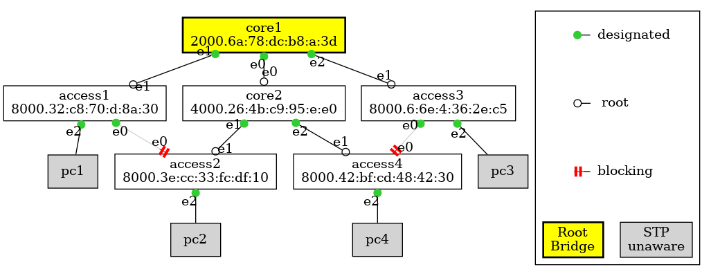
この情報をもとにDesignated PortからRoot Port、Blocking Portに線を引くとSTPトロポジの図を描くことができるのでスクリプトにしました。(一部足りない情報は別のコマンドで収集してますが)

実行するとGraphviz形式(DOT形式)の図のソースコードを標準出力に出すのと、pythonのgraphvizパッケージを使って、PNG形式の図を./output/ディレクトリに出力します。

# ./print_topology_stp_linuxbridge.py
digraph STP {
        edge [labeldistance=1.5]
        core1 [label="core1\n2000.6a:78:dc:b8:a:3d" fillcolor=yellow penwidth=2 shape=box style=filled]
        core2 [label="core2\n4000.26:4b:c9:95:e:e0" shape=box]
        access1 [label="access1\n8000.32:c8:70:d:8a:30" shape=box]
        access2 [label="access2\n8000.3e:cc:33:fc:df:10" shape=box]
        access3 [label="access3\n8000.6:6e:4:36:2e:c5" shape=box]
        access4 [label="access4\n8000.42:bf:cd:48:42:30" shape=box]
        core1 -> core2 [arrowhead=odot arrowtail=dot color="limegreen:black;0.99:black" dir=both headlabel=e0 taillabel=e0]
        core1 -> access1 [arrowhead=odot arrowtail=dot color="limegreen:black;0.99:black" dir=both headlabel=e1 taillabel=e1]
        core1 -> access3 [arrowhead=odot arrowtail=dot color="limegreen:black;0.99:black" dir=both headlabel=e1 taillabel=e2]
        core2 -> access2 [arrowhead=odot arrowtail=dot color="limegreen:black;0.99:black" dir=both headlabel=e1 taillabel=e1]
        core2 -> access4 [arrowhead=odot arrowtail=dot color="limegreen:black;0.99:black" dir=both headlabel=e1 taillabel=e2]
        access1 -> access2 [arrowhead=teetee arrowtail=dot color="limegreen:lightgray;0.99:red" dir=both headlabel=e0 taillabel=e0]
        access3 -> access4 [arrowhead=teetee arrowtail=dot color="limegreen:lightgray;0.99:red" dir=both headlabel=e0 taillabel=e0]
        pc1 [fillcolor=lightgray shape=box style=filled]
        access1 -> pc1 [arrowtail=dot color="limegreen:black;0.99:black" dir=back taillabel=e2]
        pc3 [fillcolor=lightgray shape=box style=filled]
        access3 -> pc3 [arrowtail=dot color="limegreen:black;0.99:black" dir=back taillabel=e2]
        pc2 [fillcolor=lightgray shape=box style=filled]
        access2 -> pc2 [arrowtail=dot color="limegreen:black;0.99:black" dir=back taillabel=e2]
        pc4 [fillcolor=lightgray shape=box style=filled]
        access4 -> pc4 [arrowtail=dot color="limegreen:black;0.99:black" dir=back taillabel=e2]
        subgraph cluster_legend {
                {
                        graph [rank=same]
                        h1 [label="" fixsize=true shape=none width=0]
                        designated [shape=none]
                        h1 -> designated [arrowtail=dot color="limegreen:black;0.99:black" dir=back]
                }
                {
                        graph [rank=same]
                        h2 [label="" fixsize=true shape=none width=0]
                        root [shape=none]
                        h2 -> root [arrowtail=odot color="black:black;0.99:black" dir=back]
                }
                {
                        graph [rank=same]
                        h3 [label="" fixsize=true shape=none width=0]
                        blocking [shape=none]
                        h3 -> blocking [arrowtail=teetee color="red:black;0.99:black" dir=back]
                }
                {
                        graph [rank=same]
                        unaware [label="STP
unaware" fillcolor=lightgray shape=box style=filled]
                        rootbridge [label="Root
Bridge" fillcolor=yellow penwidth=2 shape=box style=filled]
                }
                h1 -> h2 [style=invis]
                h2 -> h3 [style=invis]
                h3 -> rootbridge [style=invis]
                rootbridge -> unaware [style=invis]
        }
}

rendered file:  output/STP.gv.png

STPのRoot Bridgeが変わると図のノード配置がガラッと変わるので、あらかじめノード間の相対配置をrank=sameとinvisibleなedgeで定めた以下のようなテキストファイルを用意しておいて、

base.gv

        graph [nodesep=0.6]

        {rank=same; core1; core2;}
        core1 -> access1 [style=invis]
        core1 -> access2 [style=invis]
        core2 -> access3 [style=invis]
        core2 -> access4 [style=invis]
        access1:s -> pc1 [style=invis]
        access2:s -> pc2 [style=invis]
        access3:s -> pc3 [style=invis]
        access4:s -> pc4 [style=invis]

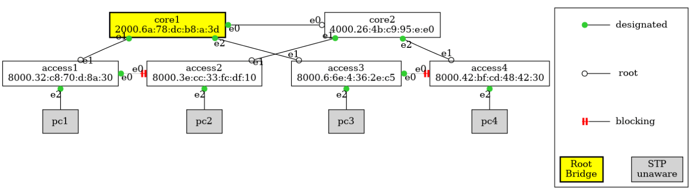
自動収集した情報をもとにDesignated Port→Root Port、Designated Port→Blocking Portの線をconstraint=false属性を付けたedgeを追加することで、ノード配置を固定したままポート状態が分かるようにもしました。^[1]

# ./print_topology_stp_linuxbridge.py -b base.gv -n -g fixed
digraph fixed {
        edge [labeldistance=1.5]
        core1 [label="core1\n2000.6a:78:dc:b8:a:3d" fillcolor=yellow penwidth=2 shape=box style=filled]
        core2 [label="core2\n4000.26:4b:c9:95:e:e0" shape=box]
        access1 [label="access1\n8000.32:c8:70:d:8a:30" shape=box]
        access2 [label="access2\n8000.3e:cc:33:fc:df:10" shape=box]
        access3 [label="access3\n8000.6:6e:4:36:2e:c5" shape=box]
        access4 [label="access4\n8000.42:bf:cd:48:42:30" shape=box]
        core1 -> core2 [arrowhead=odot arrowtail=dot color="limegreen:black;0.99:black" constraint=false dir=both headlabel=e0 taillabel=e0]
        core1 -> access1 [arrowhead=odot arrowtail=dot color="limegreen:black;0.99:black" constraint=false dir=both headlabel=e1 taillabel=e1]
        core1 -> access3 [arrowhead=odot arrowtail=dot color="limegreen:black;0.99:black" constraint=false dir=both headlabel=e1 taillabel=e2]
        core2 -> access2 [arrowhead=odot arrowtail=dot color="limegreen:black;0.99:black" constraint=false dir=both headlabel=e1 taillabel=e1]
        core2 -> access4 [arrowhead=odot arrowtail=dot color="limegreen:black;0.99:black" constraint=false dir=both headlabel=e1 taillabel=e2]
        access1 -> access2 [arrowhead=teetee arrowtail=dot color="limegreen:lightgray;0.99:red" constraint=false dir=both headlabel=e0 taillabel=e0]
        access3 -> access4 [arrowhead=teetee arrowtail=dot color="limegreen:lightgray;0.99:red" constraint=false dir=both headlabel=e0 taillabel=e0]
        pc1 [fillcolor=lightgray shape=box style=filled]
        access1 -> pc1 [arrowtail=dot color="limegreen:black;0.99:black" constraint=false dir=back taillabel=e2]
        pc3 [fillcolor=lightgray shape=box style=filled]
        access3 -> pc3 [arrowtail=dot color="limegreen:black;0.99:black" constraint=false dir=back taillabel=e2]
        pc2 [fillcolor=lightgray shape=box style=filled]
        access2 -> pc2 [arrowtail=dot color="limegreen:black;0.99:black" constraint=false dir=back taillabel=e2]
        pc4 [fillcolor=lightgray shape=box style=filled]
        access4 -> pc4 [arrowtail=dot color="limegreen:black;0.99:black" constraint=false dir=back taillabel=e2]
        subgraph cluster_legend {
                {
                        graph [rank=same]
                        h1 [label="" fixsize=true shape=none width=0]
                        designated [shape=none]
                        h1 -> designated [arrowtail=dot color="limegreen:black;0.99:black" dir=back]
                }
                {
                        graph [rank=same]
                        h2 [label="" fixsize=true shape=none width=0]
                        root [shape=none]
                        h2 -> root [arrowtail=odot color="black:black;0.99:black" dir=back]
                }
                {
                        graph [rank=same]
                        h3 [label="" fixsize=true shape=none width=0]
                        blocking [shape=none]
                        h3 -> blocking [arrowtail=teetee color="red:black;0.99:black" dir=back]
                }
                {
                        graph [rank=same]
                        unaware [label="STP
unaware" fillcolor=lightgray shape=box style=filled]
                        rootbridge [label="Root
Bridge" fillcolor=yellow penwidth=2 shape=box style=filled]
                }
                h1 -> h2 [style=invis]
                h2 -> h3 [style=invis]
                h3 -> rootbridge [style=invis]
                rootbridge -> unaware [style=invis]
        }
        graph [nodesep=0.6]

        {rank=same; core1; core2;}
        core1 -> access1 [style=invis]
        core1 -> access2 [style=invis]
        core2 -> access3 [style=invis]
        core2 -> access4 [style=invis]
        access1:s -> pc1 [style=invis]
        access2:s -> pc2 [style=invis]
        access3:s -> pc3 [style=invis]
        access4:s -> pc4 [style=invis]
}

rendered file:  output/fixed.gv.png

Bridge IDの変更

Bridge IDを変更してaccess1とaccess2、およびaccess3とaccess4の間をフォワーディング状態にすることを考えます。
access2のRoot Portはcore2に向いています。これをaccess1に向くように変更します。

Root Portを決めるときはまずRoot Path Costを見ます。今回はどちらも4で同じです。次にBPDUの送り元のBridge IDを見ます。core2は4000.26:4b:c9:95:e:e0、access1は8000.32:c8:70:d:8a:30です。

access1とaccess4のBridge Priorityを0x8000から変更して0x4000より低い数値にすれば優先度が上がりそうですね。

ip link set access1 type bridge priority 0x3000
ip link set access3 type bridge priority 0x3000

acccess2がaccess1から受け取っているBPDUです。変更後に想定通り0x3000になっていることが分かります。
変更前

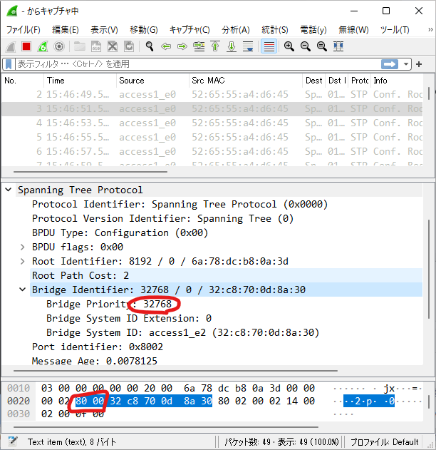
変更後

STPトポロジも確認してみます。

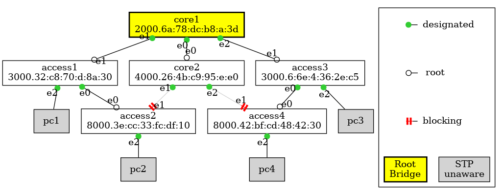
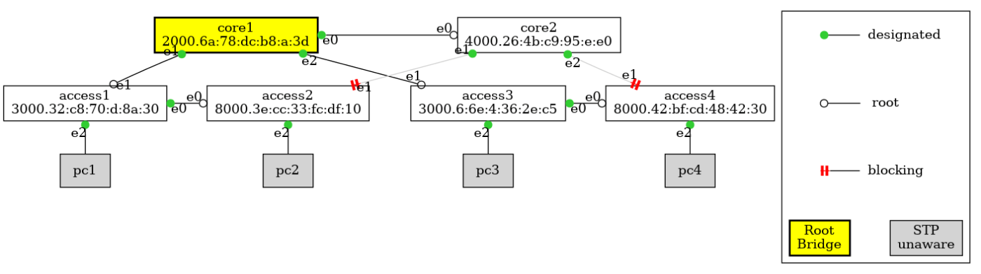
無事に思った通りのトポロジになりました。
ただ、そもそもなぜcore1のBridge Priorityを0x2000に、core2のBridge Priorityを0x4000にしているのかを考えると、この系のRoot Bridgeをcore1にするため、core1が故障時のRoot Bridgeをcore2にするためなんですよね。
(詳しくはこちら)

access1とaccess3の優先度を上げてしまった(Priority値を下げてしまった)ために、core1が故障したときにはaccess1 or access3がRoot Bridgeになる^[2]構成になってしまいました。
ですので、設計としてはこのやり方はボツですね。

Bridge Priorityは元に戻しましょう。

ip link set access1 type bridge priority 0x8000
ip link set access3 type bridge priority 0x8000

まとめ

Bridge Priorityの変更でRoot Portを変更できるか試してみました。変更できることはできるのですが、Root Bridgeの順位が変わってくるので、あんまりいい方法じゃないですね。

脚注

Graphvizでconstraint=false属性を指定すると、ノード間の相対位置(ランク)に影響を与えずにedge(線)だけを引くことができます。 ↩︎
例示している公正だとMACアドレスの差でaccess3がRoot Bridgeになります。 ↩︎

前回のおさらい

STPトポロジの可視化

Bridge IDの変更

まとめ

Discussion