⛳

microsoft/LightGBM（CLI）をElixirから使ってみる

2022/12/02に公開

Elixir

tech

この記事はElixir Advent Calendar 2022の１つです。カレンダーも是非ご覧ください！

データのクラス分類/回帰分析を行えるAI技術であるmicrosoft/LightGBMをElixirで試用する方法の紹介です。

今回はCLIを使います。

LightGBM CLIのインストール

公式サイトをみるのが一番です。必要に応じて参照してください。

Livebook上で試す

手元で軽く試すにはLivebookを使います。
まず、Dockerなどを使ってサクッと起動します。

docker run --rm -p 8080:8080 -p 8081:8081 --pull always livebook/livebook

参考：公式GitHub

新しいノートブックを開いたら、Notebook dependencies and setup 欄でインストールします。

lightgbm_cmd = File.cwd!() <> "/LightGBM/lightgbm"
if System.find_executable(lightgbm_cmd) do
  "already existing"
else
  System.shell("git clone --recursive https://github.com/microsoft/LightGBM")
  System.shell("cd LightGBM && mkdir build && cd build && cmake .. && make -j4")
end

Mix.install([
  {:scidata, "~> 0.1.9"},
  {:kino_vega_lite, "~> 0.1.5"}
])

少し時間がかかります
上記処理でのリポジトリはLIVEBOOK_DATA_PATHの直下にダウンロードされます
- 例えば、Dockerコンテナを-v $(pwd):/dataオプションで起動した場合は、LIVEBOOK_DATA_PATH=/dataがデフォルトのためpwdになります
scidataはデータセットを提供しているパッケージで、後ほど使います

LightGBM CLIの実行方法

LightGBM CLIは、設定ファイルを指定して実行する形を取ります。

例： ./lightgbm config=your_config_file other_args ...

データもCSVファイルとして用意し、そのパスを設定ファイル中で指定します。

参考：公式サイト：クイックスタート

Livebook上で試す

インストール時に取得済みの公式リポジトリにサンプルがあるので、とりあえず１つ動かしてみます。

example_dir = Path.join([File.cwd!(), "LightGBM", "examples", "regression"])

System.shell("cd #{example_dir} && #{lightgbm_cmd} config=train.conf")
System.shell("cd #{example_dir} && #{lightgbm_cmd} config=predict.conf")

結果もファイルに格納されます。

File.exists?(Path.join(example_dir, "LightGBM_predict_result.txt"))

エラーがでなければオーケーです。

以降はLivebook上でクラス分類してみた記録です。

アイリス（Iris）データセットのクラス分類

アイリスデータセットを例にとって、クラス分類の流れを試します。
必要なものは下記のとおりです。

訓練用データファイル
- 今回はCSV形式で作成します (train.csv)
訓練用設定ファイル (train.conf)
分類対象データファイル
- 今回はCSV形式で作成します (predict.csv)
分類用設定ファイル (predict.conf)

データファイルの作成

データをscidataパッケージで取得して、それぞれ書き込みます。
取得したデータはすべてクラスが既知ですが、今回は記事都合のため、訓練用と分類用（未知データ扱い）で 9:1 に分割しています。

# Irisデータの取得（および、シャッフルしたいのでそのための準備）
workdir = File.cwd!()
{features, labels} = Scidata.Iris.download()
data_size = Enum.count(labels)
prediction_size = div(data_size, 10)
shuffled_indexes = Enum.shuffle(0..(data_size - 1))
[train_indexes, prediction_indexes] = Enum.chunk_every(shuffled_indexes, data_size - prediction_size)

# 訓練用データの書き込み
train_path = Path.join(workdir, "iris_train.csv")
{train_features, train_labels} =
  Enum.reduce(train_indexes, {[], []}, fn index, {acc_x, acc_y} ->
    x = Enum.at(features, index)
    y = Enum.at(labels, index)
    {acc_x ++ [x], acc_y ++ [y]}
  end)
train_csv =
  Enum.zip(train_labels, train_features)
  |> Enum.map(& [elem(&1, 0)] ++ elem(&1, 1))
  |> Enum.map(& Enum.join(&1, ","))
  |> Enum.join("\n")
File.write!(train_path, train_csv)

# 分類用データの書き込み
# - 分類用のためfeaturesのみ必要
prediction_path = Path.join(workdir, "iris_predict.csv")
{prediction_features, prediction_labels} =
  Enum.reduce(prediction_indexes, {[], []}, fn index, {acc_x, acc_y} ->
    x = Enum.at(features, index)
    y = Enum.at(labels, index)
    {acc_x ++ [x], acc_y ++ [y]}
  end)
prediction_csv =
  prediction_features
  |> Enum.map(& Enum.join(&1, ","))
  |> Enum.join("\n")
File.write!(prediction_path, prediction_csv)

CSV仕様のノート

数値かあるいは数値化できる文字列しか扱えません
- そのため、ラベルも数値化する必要があります
- また、ラベルは0からの連番である必要があります
- ただし、例外として欠落値(missing value)をNAで記述できます
要素数が1つしかないものはCSVとしてうまく認識してくれないようです
- 訓練用はラベルがあるので問題ありませんが、分類時にエラーになりました

設定ファイルの作成

訓練用と分類用で、それぞれ作成します。特に訓練用はLightGBMのパラメータを諸々設定する必要があります。
パラメータの詳細は公式サイトをみてください。

# 訓練用
train_conf_file = Path.join(workdir, "iris_train_conf.txt")
model_file = Path.join(workdir, "iris_model.txt")

"""
task = train
data = #{train_path}
output_model = #{model_file}
label_column = 0

objective = multiclass
metric = multi_logloss
num_class = 3
num_iterations = 10
num_leaves = 5
min_data_in_leaf = 1
force_row_wise = true
saved_feature_importance_type = 1
"""
|> then(& File.write!(train_conf_file, &1))

# 分類用
prediction_conf_file = Path.join(workdir, "iris_prediction_conf.txt")
result_file = Path.join(workdir, "iris_result.tsv")

"""
task = prediction
data = #{prediction_path}
input_model = #{model_file}
output_result = #{result_file}
"""
|> then(& File.write!(prediction_conf_file, &1))

LightGBMのモデル構築と実行

やっと準備が整いました。実行してみます。

System.shell("#{lightgbm_cmd} config=#{train_conf_file}")
System.shell("#{lightgbm_cmd} config=#{prediction_conf_file}")

File.exists?(result_file)

分類結果はTSVファイルに保存されます
分類結果は各クラスの確率という形で出力されます

結果読み込み

せっかくなので結果を読み込んで正解率を確認します。

# 結果を読み込み
# // 補足：必要に応じて別途ライブラリを使ってください
results =
  result_file
  |> File.read!()
  |> String.split("\n")
  |> Enum.reject(& &1 == "")
  |> Enum.map(fn row ->
    String.split(row, "\t")
    |> Enum.map(& String.to_float/1)
  end)

# 結果の処理、最も大きい確率になったラベルを調べる
# // 補足：Nxを使うともっとシンプルにできそうです
predicted_labels =
  Enum.map(results, fn probs ->
    max = Enum.max(probs)
    Enum.find_index(probs, & &1 == max)
  end)
num_corrects =
  Enum.zip(prediction_labels, predicted_labels)
  |> Enum.count(fn {l1, l2} -> l1 == l2 end)

(num_corrects / prediction_size)
|> Float.round(2)

手元では 0.93 でした。良さそうですね（完）

蛇足ですが、Livebookの強みを活かして訓練データと分類したデータのクラス分布をみてみます。

とはいえ、特徴量が多次元なのでそのままでは可視化できません。
そこで、ここでは次元を絞ってみてみます。モデルが保存されているファイル（iris_model.txt）をみると、特徴量の重要度（feature_importances）が記録されています。

feature_importances:
Column_2=975
Column_3=198
Column_0=11
Column_1=9

いい具合に値が極端なので、よく使われているColumn_2(x3)とColumn_3(x4)で分布をみることにします。

まずはグラフ描画の準備をします。

{train_x3, train_x4} =
  train_features
  |> Enum.reduce({[], []}, fn row, {acc_x3, acc_x4} ->
    {acc_x3 ++ [Enum.at(row, 2)], acc_x4 ++ [Enum.at(row, 3)]}
  end)

{prediction_x3, prediction_x4} =
  prediction_features
  |> Enum.reduce({[], []}, fn row, {acc_x3, acc_x4} ->
    {acc_x3 ++ [Enum.at(row, 2)], acc_x4 ++ [Enum.at(row, 3)]}
  end)

x3_min = Enum.min(train_x3 ++ prediction_x3)
x3_max = Enum.max(train_x3 ++ prediction_x3)
x4_min = Enum.min(train_x4 ++ prediction_x4)
x4_max = Enum.max(train_x4 ++ prediction_x4)

new_scatter = fn x, y, class ->
  VegaLite.new(width: 300, height: 300)
  |> VegaLite.data_from_values(x: x, y: y, class: class)
  |> VegaLite.mark(:point)
  |> VegaLite.encode_field(:x, "x",
    type: :quantitative,
    scale: [domain: [x3_min, x3_max]],
    title: "Column_2"
  )
  |> VegaLite.encode_field(:y, "y",
    type: :quantitative,
    scale: [domain: [x4_min, x4_max]],
    title: "Column_3"
  )
  |> VegaLite.encode_field(:color, "class", type: :nominal)
end
:ok

準備ができたのでそれぞれの散布図を確認してみます。
最初に、訓練データの散布図を表示してみます。

new_scatter.(train_x3, train_x4, train_labels)

訓練データの分布

次に、分類対象データのモデル出力と正解データの散布図を表示してみます。

VegaLite.new(width: 300*2, height: 300)
|> VegaLite.concat([
  # モデル出力データ
  new_scatter.(prediction_x3, prediction_x4, predicted_labels),
  # 正解データ
  new_scatter.(prediction_x3, prediction_x4, prediction_labels)
], :horizontal)

分類対象データの分布

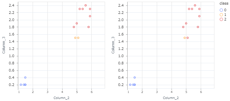
なるほど。（雑ですが）この2つの特徴だけでみると、モデル出力が間違えたところは人がみても判断が難しそうなところですね。

補足：過学習の防止（アーリーストッピング）

アーリーストッピング(early_stopping)と呼ばれる仕組みがあります。これは、訓練用データに過度にフィットするモデルができないように、ブレーキをかけるための仕組みです。

具体的には、訓練に使わない検証データを用意して、検証データに対する分類結果が悪化していくような段階で訓練をやめる、という考え方です。

LightGBM CLIでも、アーリーストッピングの検証用データもファイルとして用意しておくことで利用可能です。

結び

著者は、ElixirからPythonを経由してLightGBMを使ったりしていましたが、手元ではCLIを使った方が速度面で優位でした。前処理もNxをはじめとしたパッケージが充実しており、（私の用途では）Pythonとはおさらばできそうです。

面倒な処理を省くためにラッパーライブラリを作ってみたので、そちらを使う記事も書きました。ご覧ください。

LightGBM CLIのインストール

Livebook上で試す

LightGBM CLIの実行方法

Livebook上で試す

アイリス（Iris）データセットのクラス分類

データファイルの作成

設定ファイルの作成

LightGBMのモデル構築と実行

結果読み込み

補足：過学習の防止（アーリーストッピング）

結び

Discussion