MATLABMobileのログデータをなるべく簡潔に料理する.~加速度のログから距離の算出まで~
はじめに
MATLABMobileで取得した加速度や角速度のデータから,移動距離や方向を算出する.
なるべくfor文や自作関数を使用せず,簡潔になるようにしてみる.
MATLAB Mobileの概要や使い方についてはMATLAB Mobile でのセンサー データの収集参照.
また,今回のデータ・プログラム一式は下記リポジトリにある.
または下記のアイコンをクリックすると,直接MATLABが開ける(多分要アカウント).
なお,試行錯誤の後が残っているのでご容赦ください.

データ収集
手元に姫路から新大阪までを新幹線で移動した際のデータ(データ名:himeji2shinosaka.mat)があるので,それを利用する.
なお,全データは膨大なのと,途中停車駅でのドリフト誤差が累積されてしまうので(後述),姫路西明石間のみ取り出す.
新幹線を選択した理由
新幹線は下記の点でデータ処理がしやすいと考えた.
- 窓際の席にちょうどいいスマホを置くスペースがある.
- 加速性能が良いのでわかりやすい.
- 線路の継ぎ目が少なく,振動が少ない.また高架なので安定している.
- 線形が直線に近く,カーブの曲率も大きい.
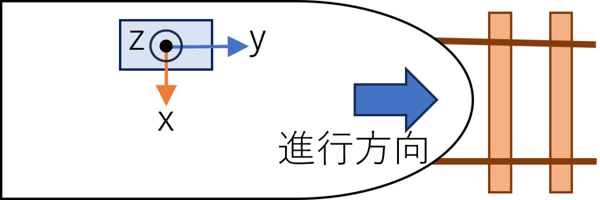
座標系
MATLABMobileをインストールしたスマホを窓際のスペースにおいてログを取得した.
センサの座標系と列車の関係は下図の通り.
データの料理
ログデータの読み込み
ログデータを読み込む.
MATLABMobileのログデータはtimetableとして読み込まれる.
% センサーデータの読み込み
load("himeji2shinosaka.mat")
つぎに読み込んだデータを一つにまとめる.
今回は測定できるログはすべて取っており,使わないものもまとめて一つにする.
timetableの合体の仕方は以前の記事参照.
sensor = synchronize(Acceleration,AngularVelocity,MagneticField,Orientation,Position,'union','previous');
sensor = rmmissing(sensor);
% 時間を初期値を0にする
sensor.Timestamp = sensor.Timestamp-sensor.Timestamp(1);
%センサーの時間切り出し
sensor = sensor(1:200000,:);
データの整形とプロットでの確認
加速度
加速度についてデータを観る.
まず,加速度データを取り出して一つの配列にする.
Acc = [sensor.X_Acceleration,sensor.Y_Acceleration,sensor.Z_Acceleration];
センサ値にはバイアスが乗っているので,最初の500個の平均値をもとめ,データから引く.
% バイアスの確認
AccBias = mean(Acc(1:500,:));
% バイアスの修正
Acc = Acc-AccBias;
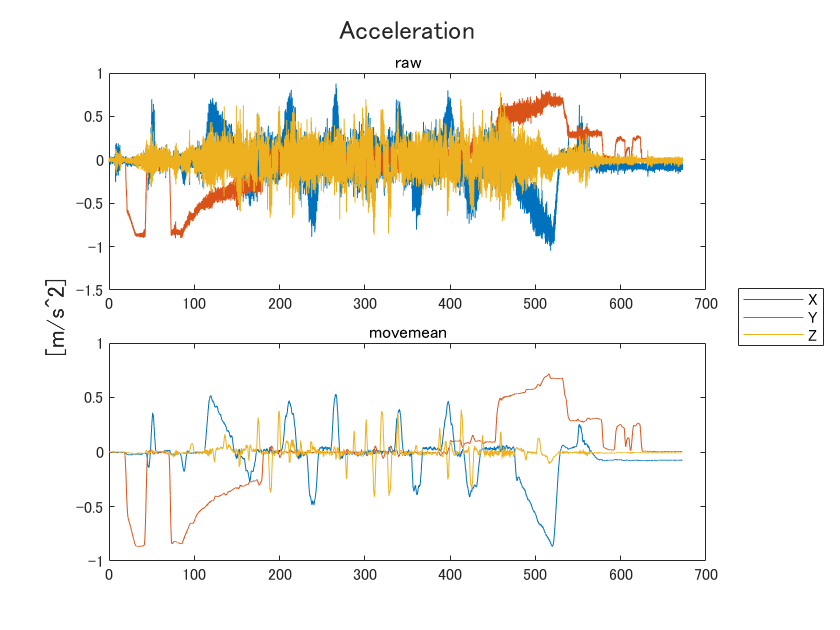
上記のままではノイズが多く後段での処理にノイズの影響が多く出てしまうので,今回は移動平均をとってセンサ値を滑らかにする.
移動平均はmovmean関数を使用すると簡単に取得できる.
movmeanAcc = movmean(Acc,windowsize);
加速度データをプロットすると下図のようになり,移動平均をとると高周波成分が減って見やすくなる.
速度と位置
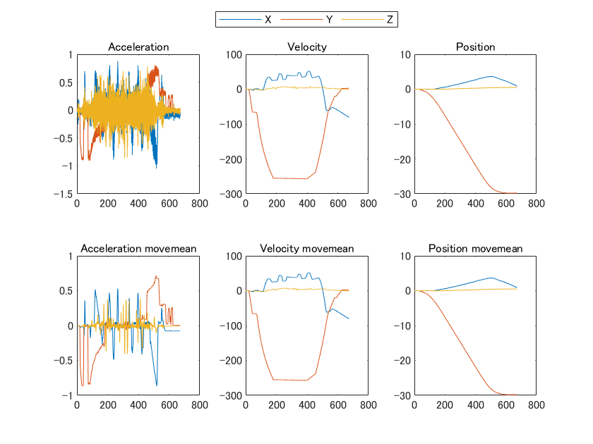
加速度データを積分することにより,速度を算出できる.
今回は台形積分を用いる.
台形積分を用いると,離散値の関数
これを愚直にプログラムすると,時間ステップの差分をとってfor文で0から1ステップずつ計算して…
となるが,MATLABにはなんとこれを一発でやってしまうcumtrapz関数がある.
これを使うと,速度は下記のように計算できる.
% 速度
Vel = cumtrapz(secondsTime,Acc,1);
% 移動平均加速度を積分する場合
movmeanVel = cumtrapz(secondsTime,movmeanAcc,1);
一つ目の引数はサンプル点(省略可,省略すると間隔1として扱われる),二つ目の引数はサンプル点での値,三つ目の引数は列方向に適用するということを示す.
なお,最終値のみほしい場合はtrapz関数があり,引数は同じである.
同様にして速度を台形積分すると位置が得られる.
% 位置
Pos = cumtrapz(secondsTime,Vel,1);
% 移動平均速度を積分する場合
movmeanPos = cumtrapz(secondsTime,movmeanVel,1);
加速度,速度,位置をまとめてプロットすると下図のようになる.
座標軸の関係で正負が変わっているが,きちんと積分値が得られていることが確認できる.
プロットのコード
tiledlayoutを使うと便利.
% まとめのプロット
figure
tiledlayout(2,3)
% 加速度
nexttile;
plot(secondsTime,Acc)
title("Acceleration")
% 速度
nexttile;
plot(secondsTime,Vel*3600/1000)
title("Velocity")
% 位置
nexttile;
plot(secondsTime,Pos/1000)
title("Position")
% 移動平均
% 加速度
nexttile;
plot(secondsTime,movmeanAcc)
title("Acceleration movemean")
% 速度
nexttile;
plot(secondsTime,Vel*3600/1000)
title("Velocity movemean")
% 位置
nexttile;
plot(secondsTime,movmeanPos/1000)
title("Position movemean")

lgd = legend(["X","Y","Z"],'Orientation', 'horizontal','Location','north');
lgd.Layout.Tile = 'north';
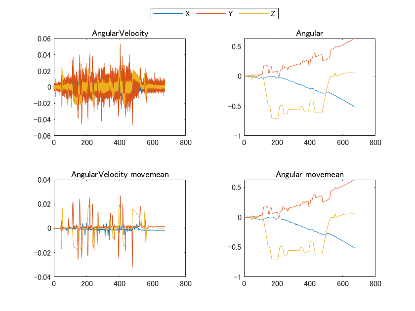
角速度と角度
角速度についても同様にまとめてプロットする.
結果を示すと下図のようになり,角度は捉えられているが,角度データにドリフトが乗ってそうなことがわかる.
なお,ドリフトを取り除くにはdetrend等が使用できるが,今回は使っていない.
コード
windowsize = 500;
secondsTime = seconds(sensor.Timestamp);
% 角度まとめる
AngVel = [sensor.X_AngularVelocity,sensor.Y_AngularVelocity,sensor.Z_AngularVelocity];
% バイアスの確認
AngVelBias = mean(AngVel(1:500,:));

% 角速度のバイアス修正
AngVel = AngVel-AngVelBias;
%トレンドの修正
% X_AngVel = detrend(X_AngVel,1);
% Y_AngVel = detrend(Y_AngVel,1);
% Z_AngVel = detrend(Z_AngVel,1);

figure
tiledlayout(2,2);
nexttile;
plot(secondsTime,AngVel)
title("AngularVelocity")
%角度変化
nexttile
Ang = cumtrapz(secondsTime,AngVel,1);
plot(secondsTime,Ang)
title("Angular")

%移動平均のプロット
nexttile;
movmeanAngVel = movmean(AngVel,windowsize);
plot(secondsTime,movmeanAngVel)
title("AngularVelocity movemean")
nexttile;
movmeanAng = cumtrapz(secondsTime,movmeanAngVel,1);
plot(secondsTime,movmeanAng)
title("Angular movemean")

lgd = legend(["X","Y","Z"],'Orientation', 'horizontal','Location','north');
lgd.Layout.Tile = 'north';
地図上へのプロット
移動距離を緯度と経度に変換し,地図上にプロットする.
角度のデータを元に,オイラー角を取得する.Z-Y-X回転で変換する.
なお,小数点の数字は,試行錯誤的に合わせた数値である.
rotmZYX = eul2rotm([-movmeanAng(:,3)+pi/2+0.15,-movmeanAng(:,2)+0.2,-movmeanAng(:,1)-0.2]);
これにより回転行列の
この回転行列に加速度のデータ(
各ステップごとにpagemtimes関数を使うと一度に計算できる.
なお,関数を適用するために,permuteで並び変えて適用したあと,元に戻す.
movmeanAcc2 = pagemtimes(rotmZYX,permute(movmeanAcc,[2,3,1]));
movmeanAcc2 = permute(movmeanAcc2,[3,1,2]);
この座標変換後の値を前節と同じように積分すると位置が得られる.
これを緯度経度にするには,地球を半径
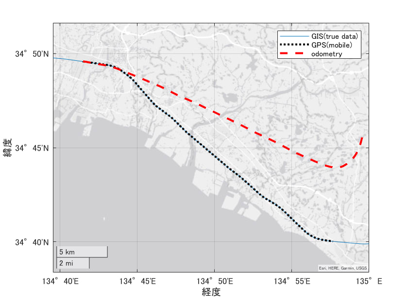
以上の処理により緯度と経度が得られるので,これを地図上にプロットすると下図.
なお,センサで測定したGPS座標と,国交省の鉄道の数値データを合わせてプロットしている.
国交省の数値データプロット方法は以前の記事参照.
コード
% 回転
rotmZYX = eul2rotm([-movmeanAng(:,3)+pi/2+0.15,-movmeanAng(:,2)+0.2,-movmeanAng(:,1)-0.2]);

movmeanAcc2 = pagemtimes(rotmZYX,permute(movmeanAcc,[2,3,1]));
movmeanAcc2 = permute(movmeanAcc2,[3,1,2]);
% Y方向の反転
movmeanAcc2(:,2) = -movmeanAcc2(:,2);

figure
tiledlayout(1,3);
% 加速度
nexttile;
plot(secondsTime,movmeanAcc2)
legend(["X","Y","Z"])
title("Acceleration_movemean")
% 速度
nexttile;
movmeanVel = cumtrapz(secondsTime,movmeanAcc2,1);
plot(secondsTime,movmeanVel*3600/1000)
legend(["X","Y","Z"])
title("Velocity_movemean")
% 位置
nexttile;
movmeanPos = cumtrapz(secondsTime,movmeanVel,1);
plot(secondsTime,movmeanPos/1000)
legend(["X","Y","Z"])
title("Position_movemean")

% 距離から緯度経度の計算
% 一ステップ間で経度計算時は緯度は一定とする,
% 地球は球面とする.地球半径R=6378137m
% 緯度の差分:rad2deg(Y方向移動[m]/R)
% 経度の差分:rad2deg(x方向移動/r) ,ただしr = R*cos(緯度)
initLatitude = sensor.latitude(1);
initLongtitude = sensor.longitude(1);
R = 6378137;
% 緯度方向の計算
odomLatitude = rad2deg(movmeanPos(:,2)/R) + initLatitude;
odomLongtitude = rad2deg(movmeanPos(:,1)./(R*cosd(odomLatitude))) + initLongtitude;

%% geoplot
figure
gx = geoaxes;
hold(gx);
%% GISデータのプロット
txt = readlines("N02-19_RailroadSection.geojson");
txt = strrep(txt,'鉄道区分','railsegments');
txt = strrep(txt,'事業者種別','companysegments');
txt = strrep(txt,'路線名','railname');
txt = strrep(txt,'運営会社','company');
geojson = jsondecode(strjoin(txt))
% 山陽新幹線
railname = ["山陽新幹線"];
company = ["西日本旅客鉄道"];
color = ["#0072BA"];

for ii=1:length(railname)
    plotCoordinate(gx,geojson,railname(ii),company(ii),color(ii))
end

% ログデータのプロット
geoplot(gx,sensor.latitude,sensor.longitude,'k:',LineWidth=2)
geoplot(gx,odomLatitude,odomLongtitude,'r--',LineWidth=2)
hold off
legend(["GIS(true data)","GPS(mobile)", "odometry"])
geolimits([34.64 34.86],[134.659 135.00])

%% 関数
function plotCoordinate(gx,geojson,railName,company,color)
    railcoordinate = [];
        for ii=1:length(geojson.features)
        if string(geojson.features(ii).properties.railname)==railName && string(geojson.features(ii).properties.company)==company
            railcoordinate = [railcoordinate;geojson.features(ii).geometry.coordinates];
        end
        end
        railcoordinate = sortrows(railcoordinate);
        geoplot(gx,railcoordinate(:,2),railcoordinate(:,1),"Color",color);
end
赤破線が加速度データからの位置であるが,実際の位置と比べて誤差がどんどん出ている....
また,赤破線の右の端で上に向かって線が伸びているが,これは西明石駅での停車時に角速度にドリフトが乗っていて,それが累積された結果と思われる.
これにより,全経路でプロットするとどんどんあらぬ方向に進んでしまうので今回は姫路から西明石までとしている.
窓際に置いただけなので置き場所の傾きなどがあり,オドメトリ計算するのはやはり困難...センサはしっかり固定しないとだめですね.
おわりに
MATLABMobileでデータをとりそのまま使えるのは楽しい.
もっといろいろな処理がありそうなので試してみるのもいいかもしれない.
カルマンフィルタをかませるのも一つの手にはなるが,プロット見る限りGPSが優秀なので面白い結果が得られるかどうか...?
関数や処理をゴリゴリ自作するのもいいけれど,望む処理ができる関数を探してスマートにつかうのも知識が広がる感じがして良い.
姫路から新大阪までの間のデータは上部のリポジトリに置いているので,試したい人はどうぞ使ってみてください.
Discussion