[統計学]モンテカルロ積分の証明と実践

概要

モンテカルロ積分の証明を忘れていたことに気づいたので証明を行う. モンテカルロ積分とは乱数を用いた積分手法である.

定義・性質

以下の積分を確率変数を用いて行うことを考える

• 関数: $g(x)$.
• 積分: $\theta = \int_0^1 g(x) dx$.
• 確率変数: $X : X \backsim U(0,1)$.

このとき, $\theta$ について以下が成り立つ.

$$\mathbb{E}[g(X)] = \int_0^1 g(x) \cdot \frac{1}{1-0} dx = \theta.$$

すなわち, $\mathbb{E}[g(X)]$ を推定すればよい. ここで以下の無作為標本を考える.

• $X_1, \cdots ,X_m \quad \text{Where} \quad X_i \backsim U(0,1)$.

このとき以下の確率収束が成り立つ.

$$\begin{align*} \hat{\theta} &= \frac{1}{m} \sum_{i=1}^m g(X_i) \\ \plim_{m \rightarrow \infty} \hat{\theta} &\rightarrow\theta \end{align*}$$

上記の式を用いて $\theta$ を推定する方法をモンテカルロ積分という. 便宜上区間$(0,1)$にしているが, 積分区間が異なる場合は確率密度を計算して調整することで計算ができる.

証明

いくつかポイントがあるのでそれらを順に解説する.

大数の弱法則が成り立てば確率収束が成立することを確認する.

まず, 下記の式が成り立つ理由だが, これは大数の弱法則(weak law of large numbers))を用いている.

$$\begin{align*} \hat{\theta} &= \frac{1}{m} \sum_{i=1}^m g(X_i) \\ \plim_{m \rightarrow \infty} \hat{\theta} &\rightarrow\theta \end{align*}$$

大数の弱法則は以下の式である.

$$\begin{align*} &\forall \epsilon > 0, \lim_{m \rightarrow \infty} P(|\bar{X} - \mu| \geq \epsilon) = 0. \\ &\text{Where,}\quad \bar{X} = m^{-1} \sum_{i=1}^m X_i. \end{align*}$$

よってこの法則が成り立てばモンテカルロ積分の確率収束は成り立つ.

大数の弱法則が成り立つことを確認する

大数の弱法則が成り立てば積分の近似ができることがわかったのでこの法則が成り立つことを確認する. ここで, $\bar{X}$ の期待値・分散は$X_i$ が無作為標本であることから, 下記が成り立つことに注意.

$$\begin{align*} \mathbb{E}[\bar{X}] &= \mathbb{E}[m^{-1}\sum_{i=1}^m X_i] \\ &= m^{-1}\sum_{i=1}^m\mathbb{E}[X_i] \\ &= m^{-1}\sum_{i=1}^m \mu \\ &= \mu. \\ \mathbb{V}[\bar{X}] &= \mathbb{V}[m^{-1}\sum_{i=1}^m X_i] \\ &= m^{-2}\sum_{i=1}^m\mathbb{V}[X_i] \\ &= m^{-2}\sum_{i=1}^m \sigma^2 \\ &= m^{-1}\sigma^2. \end{align*}$$

ここで下記のチェビシェフの不等式と呼ばれる式が成り立つとする.

$$P(|X-\mu| \geq \epsilon) \leq \sigma^2 \epsilon^{-2}.$$

この式に$\bar{X}$ を入れると右辺の分散が$m^{-1} \sigma^2$ であることから, $\lim m \rightarrow \infty$ において任意の$\epsilon > 0$ について以下が成り立つ.

$$\lim_{m \rightarrow \infty} P(|\bar{X} - \mu| \geq \epsilon) = 0.$$

この式は大数の弱法則の式そのものである.

チェビシェフの不等式が成り立つことを確認する

これまでの議論からチェビシェフの不等式が成り立つことが示せば, 大数の弱法則が成り立ち, モンテカルロ積分も成り立つ. そこでチェビシェフの不等式を証明する. 尚, 便宜上確率変数は連続確率変数を仮定する.

まず, 以下の式が成り立つことを確認する.

$$\begin{align*} \mathbb{E}[|X|] &= \int_{-\infty}^{\infty} |x| f(x)dx \\ &\geq \int_{|x| \geq \epsilon} |x| f(x)dx \\ &\geq \int_{|x| \geq \epsilon} \epsilon f(x)dx \\ &= \epsilon P(|x| \geq \epsilon) \\ \\ \text{Where}& \quad 0 < \epsilon \end{align*}$$

• 第二行は積分範囲を制限しているので不等式が成り立つ.
• 第三行は積分区間の条件より明らかに不等式が成り立つ.
• 第四行は定数を外に出して残った積分の部分を確率の表記に直している.
• (尚, この式をマルコフの不等式という.)

この式に$|X-\mu|^2$ を入れると以下のようになる.

$$\begin{align*} \mathbb{E}[|X-\mu|^2] &= \int_{-\infty}^{\infty} |x-\mu| ^2f(x)dx \\ &\geq \int_{|x-\mu| \geq \epsilon} |x-\mu|^2 f(x)dx \\ &\geq \int_{|x-\mu| \geq \epsilon} \epsilon^2 f(x)dx \\ &= \epsilon^2 P(|x-\mu| \geq \epsilon) \\ \\ \text{Where}& \quad 0 < \epsilon \end{align*}$$

ところで, 左辺は定義より, $\sigma^2$である. 従って以下のように書き直すことができる.

$$P(|x-\mu| \geq \epsilon) = \sigma^2 \epsilon^{-2}$$

この式はチェビシェフの不等式そのものである.

まとめ

以上の議論からモンテカルロ積分が成り立つ.

モンテカルロ積分の実装

今回は$f(x) = x^2$の$(0,1)$の範囲を積分する. 真の値は$1/3$ になる.

コードは以下を参照

import numpy as np
import matplotlib.pyplot as plt
import seaborn as sns

def f(x: np.ndarray) -> np.ndarray:
    """
    Calculates the sigmoid function for a numpy array.

    Args:
    x (np.ndarray): the input array.

    Returns:
    np.ndarray: the f of the input array.
    """
    return x**2

# Generate the x values for the target function
x = np.linspace(-10, 10, 1000)

# Calculate the target function for x
y = f(x)

# Setting for plot
sns.set()
sns.set_style("whitegrid", {'grid.linestyle': '--'})
sns.set_context("talk", 0.8, {"lines.linewidth": 2})
sns.set_palette("cool", 2, 0.9)

# Plot
fig=plt.figure(figsize=(16,9))
ax1 = fig.add_subplot(1, 1, 1)
plt.plot(x, y)
plt.title('Target Function')
plt.xlabel('x')
plt.ylabel('f of x')
plt.show()

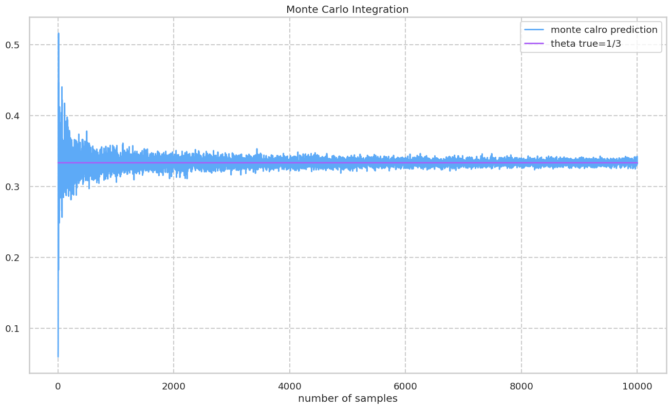
サンプリングの回数を変えてモンテカルロ積分を行い, 真の値と比較をする. 以下の図では真の値に収束する様子が確認できる.

def generate_uniform_array(n: int) -> np.ndarray:
    """
    Generates a numpy array with n elements using uniform distribution with parameter a=0 and b=1.

    Args:
    n (int): the number of elements in the array.

    Returns:
    np.ndarray: a numpy array with n elements.
    """
    arr = np.random.uniform(0, 1, n)
    return arr

def estimate_theta(num_of_samples: int) -> float:
    """
    Calculates the sigmoid function for a numpy array.

    Args:
    num_of_sumples (int): the number of sample

    Returns:
    res (float): estimated value 
    """
    tmp: np.ndarray = f(generate_uniform_array(num_of_samples))
    res: float    = float(sum(tmp)/len(tmp))
    return res

# Generate the x values and the true values
x = [i for i in range(1, 10000, 1)]
theta_true = [1/3 for i in range(len(x))]

# Estimate Integration
theta_hats = [estimate_theta(num_of_samples=i) for i in x]

# Setting for plot
sns.set()
sns.set_style("whitegrid", {'grid.linestyle': '--'})
sns.set_context("talk", 0.8, {"lines.linewidth": 2})
sns.set_palette("cool", 2, 0.9)

# Plot
fig=plt.figure(figsize=(16,9))
ax1 = fig.add_subplot(1, 1, 1)
plt.plot(x, theta_hats)
plt.plot(x, theta_true)

# write information
plt.title('Monte Carlo Integration')
plt.xlabel('number of samples')
ax1.legend(['monte calro prediction','theta true=1/3'])
plt.show()

参考文献

• hanada, matsuura.”0からできるMCMC マルコフ連鎖モンテカルロ法の実践的入門”.2020.講談社
• takemura et al.”日本統計学会公式認定 統計検定準1級対応 統計学実践ワークブック”.2020.学術図書
• takemura.”新装改訂版 現代数理統計学”.2020.学術図書
• ”Monte Carlo Integration”.25 January 2023.Wikipedia
• masuo."大数の法則をわかりやすく【意味・具体例・証明】".February 2022.高校数学の美しい物語