Python で Tellus の衛星データを検索・取得する
この記事では、tellus-traveler という Python パッケージを使って、衛星データプラットフォーム Tellus の衛星データを検索・取得する方法を紹介します。
tellus-traveler は pip を使ってインストールできます。
$ pip install tellus-traveler
API トークンをセットする
tellus-traveler は Tellus Satellite Data Traveler API を利用します。
この API の利用には API トークンが必要なため、Tellus にログインし、https://www.tellusxdp.com/account/setting/api-access/ で発行したトークンを tellus_traveler.api_key に代入してください。
import tellus_traveler

tellus_traveler.api_token = "YOUR_TELLUS_API_TOKEN"
あるいは、環境変数 TELLUS_API_TOKEN に API トークンを設定すれば、tellus-traveler はその値を自動で読みます。
全データセットのリストを取得する
Tellus の衛星データは、その種類ごとに「データセット」という単位でまとめられています。
tellus_traveler.datasets() でその全リストを取得できます。
datasets = tellus_traveler.datasets()
データセットの各要素は次のような辞書です。
import pprint

pprint.pp(datasets[0])
{'id': '1a41a4b1-4594-431f-95fb-82f9bdc35d6b',
 'provider': {'name': 'テルース', 'description': 'テルースが提供する公式データです'},
 'tags': [],
 'published_at': '2021-10-08T14:24:12.960797+09:00',
 'can_order_access_right': True,
 'can_order_cut_data': False,
 'is_order_required': False,
 'minimum_purchase_square_kilometer': 0,
 'square_kilometer_per_price': 0,
 'related_site': 'https://www.eorc.jaxa.jp/ALOS/a/jp/index_j.htm',
 'copyright': '©JAXA',
 'properties': ['sat:orbit_state',
                'sar:observation_direction',
                'view:off_nadir',
                'sar:polarizations',
                'sar:frequency_band',
                'sat:relative_orbit',
                'tellus:sat_frame',
                'sar:instrument_mode',
                'processing:level',
                'sar:product_type',
                'gsd',
                'palsar2:beam'],
 'prices': [],
 'name': '【Tellus公式】PALSAR-2_L1.1',
 'description': 'JAXAが開発したPALSAR-2というSARセンサのデータです。',
 'terms_of_use': '/api/traveler/v1/datasets/1a41a4b1-4594-431f-95fb-82f9bdc35d6b/terms-of-use-url/',
 'manual': '/api/traveler/v1/datasets/1a41a4b1-4594-431f-95fb-82f9bdc35d6b/manual-url/',
 'permission': {'allow_network_type': 'tellus'}}
ここでは、無料で Tellus 環境外でも利用できる可視域を含む光学データということで、AVNIR-2_1B1 を対象にします。
AVNIR-2 は、JAXA の人工衛星「だいち」に搭載されていたセンサです。
avnir2_dataset = next(dataset for dataset in datasets if "AVNIR-2" in dataset["name"])
pprint.pp(avnir2_dataset)
{'id': 'ea71ef6e-9569-49fc-be16-ba98d876fb73',
 'provider': {'name': 'テルース', 'description': 'テルースが提供する公式データです'},
 'tags': [],
 'published_at': '2021-10-08T14:26:06.089400+09:00',
 'can_order_access_right': True,
 'can_order_cut_data': False,
 'is_order_required': False,
 'minimum_purchase_square_kilometer': 0,
 'square_kilometer_per_price': 0,
 'related_site': 'https://www.eorc.jaxa.jp/ALOS/jp/alos/a1_about_j.htm',
 'copyright': '©JAXA',
 'properties': ['sat:orbit_state',
                'tellus:pointing_angle',
                'tellus:bands',
                'sat:relative_orbit',
                'tellus:sat_frame',
                'processing:level',
                'eo:cloud_cover',
                'gsd'],
 'prices': [],
 'name': '【Tellus公式】AVNIR-2_1B1',
 'description': '解像度10mの広域撮影を目的とした光学カラー画像です。\nJAXAのAVNIR-2センサデータから生成されています。',
 'terms_of_use': '/api/traveler/v1/datasets/ea71ef6e-9569-49fc-be16-ba98d876fb73/terms-of-use-url/',
 'manual': '/api/traveler/v1/datasets/ea71ef6e-9569-49fc-be16-ba98d876fb73/manual-url/',
 'permission': {'allow_network_type': 'global'}}
シーンを検索する
JAXA の筑波宇宙センターがある茨城県つくば市を観測した AVNIR-2 データを検索してみましょう。
「だいち」が運用停止した2011年4月を対象にします。
まず、つくば市の緯度経度の範囲(Bounding Box)を国土数値情報ダウンロードサイトから取得します。
次のコードでは GeoPandas を利用しています。
import geopandas as gpd

ibaraki_gdf = gpd.read_file("/vsizip//vsicurl/https://nlftp.mlit.go.jp/ksj/gml/data/N03/N03-2023/N03-20230101_08_GML.zip/N03-23_08_230101.geojson")
tsukuba_gdf = ibaraki_gdf[ibaraki_gdf["N03_004"] == "つくば市"]
tsukuba_bbox = tsukuba_gdf.total_bounds
pprint.pp(tsukuba_bbox)
array([139.9957985 , 35.94732097, 140.17316041, 36.23682703])
tellus_traveler.search() に検索条件を渡して呼び出します。
search = tellus_traveler.search(
    datasets=[avnir2_dataset["id"]],
    bbox=tsukuba_bbox,
    start_datetime="2011-04-01T00:00:00Z",
    end_datetime="2012-05-01T00:00:00Z",
)
pprint.pp(search.total())
4
Tellus では、個々の衛星画像を「シーン」と呼びます。
search.total() の結果より、4件のシーンが見つかったことがわかります。
tellus_traveler.search() は SceneSearch クラスのインスタンスを返します。
メソッド scenes() により、個々のシーンに対応する Scene オブジェクトが得られます。
検索結果が多い場合に適宜ページネーションするため、返り値はジェネレータになっているのですが、今回は4件なのでリストにします。
scenes = list(search.scenes())
pprint.pp(scenes)
[<tellus_traveler.Scene id=87c64a3f-0ec0-429a-b3e9-4c528cdc245c>,
 <tellus_traveler.Scene id=7b223975-9116-4d40-9665-3133ab6bdfdb>,
 <tellus_traveler.Scene id=72751033-d91b-4da8-b761-b7494a4d3213>,
 <tellus_traveler.Scene id=adfe5357-d4e2-4638-a8e6-732d37a18418>]
検索結果のシーンは GeoJSON の Feature 型になっています。
属性 __geo_interface__ で内容を確認できます。
pprint.pp(scenes[0].__geo_interface__)
{'dataset_id': 'ea71ef6e-9569-49fc-be16-ba98d876fb73',
 'geometry': {'coordinates': [[[139.9240901, 35.8359832],
                               [140.703506, 35.6882876],
                               [140.9089491, 36.3899905],
                               [140.1229063, 36.5389288],
                               [139.9240901, 35.8359832]]],
              'type': 'Polygon'},
 'id': '87c64a3f-0ec0-429a-b3e9-4c528cdc245c',
 'type': 'Feature',
 'properties': {'tellus:pointing_angle': 0.0,
                'processing:level': 'L1B1',
                'sat:relative_orbit': 67,
                'start_datetime': '2011-04-10T01:27:23.348878+00:00',
                'end_datetime': '2011-04-10T01:27:23.348878+00:00',
                'tellus:name': 'ALAV2A277442870',
                'tellus:bands': ['band1', 'band2', 'band3', 'band4'],
                'created': '2021-09-22T04:07:47.101506+00:00',
                'tellus:can_ordered': True,
                'tellus:sat_frame': 2870,
                'tellus:published_datetime': '2021-09-22T04:08:17.227940+00:00',
                'sat:orbit_state': 'descending',
                'eo:cloud_cover': 25.5,
                'gsd': 10.0,
                'updated': '2021-10-22T21:29:27.251006+00:00'}}
GeoPandas を使って、検索結果の詳細を確認してみましょう。
ここでは geopandas.GeoDataFrame.explore を使って、GUI で確認しています。
以下は画像ですが、実際には拡大・縮小や各シーンのメタデータの表示ができます。
import folium

search_results_gdf = gpd.GeoDataFrame.from_features(scenes, crs="EPSG:4326")
map = search_results_gdf.explore("tellus:name")
folium.Rectangle(bounds=[(tsukuba_bbox[1], tsukuba_bbox[0]), (tsukuba_bbox[3], tsukuba_bbox[2])]).add_to(map)
map

以降は、もっともつくば市を含む範囲が広い ALAV2A277442870 を使うことにします。
scene = next(scene for scene in scenes if scene["tellus:name"] == "ALAV2A277442870")
pprint.pp(scene.properties)
{'tellus:pointing_angle': 0.0,
 'processing:level': 'L1B1',
 'sat:relative_orbit': 67,
 'start_datetime': '2011-04-10T01:27:23.348878+00:00',
 'end_datetime': '2011-04-10T01:27:23.348878+00:00',
 'tellus:name': 'ALAV2A277442870',
 'tellus:bands': ['band1', 'band2', 'band3', 'band4'],
 'created': '2021-09-22T04:07:47.101506+00:00',
 'tellus:can_ordered': True,
 'tellus:sat_frame': 2870,
 'tellus:published_datetime': '2021-09-22T04:08:17.227940+00:00',
 'sat:orbit_state': 'descending',
 'eo:cloud_cover': 25.5,
 'gsd': 10.0,
 'updated': '2021-10-22T21:29:27.251006+00:00'}
ファイルをダウンロードする
Scene.file() や Scene.thumbnail() で対象のシーンのファイルやサムネイルの情報を取得できます。
files = scene.files()
pprint.pp(files)

thumbs = scene.thumbnails()
pprint.pp(thumbs)
[{'size_bytes': 1784,
  'mime_type': 'text/plain',
  'name': 'HDR-ALAV2A277442870-OORIRFU-D067P3-20110410-002.txt',
  'id': 1,
  'status': 'uploaded',
  'is_downloadable': True,
  'require_archived_file_download': False},
 {'size_bytes': 85203240,
  'mime_type': 'image/tiff',
  'name': 'IMG-04-ALAV2A277442870-OORIRFU-D067P3-20110410-002.tif',
  'id': 2,
  'status': 'uploaded',
  'is_downloadable': True,
  'require_archived_file_download': False},
 {'size_bytes': 85203240,
  'mime_type': 'image/tiff',
  'name': 'IMG-03-ALAV2A277442870-OORIRFU-D067P3-20110410-002.tif',
  'id': 3,
  'status': 'uploaded',
  'is_downloadable': True,
  'require_archived_file_download': False},
 {'size_bytes': 85203240,
  'mime_type': 'image/tiff',
  'name': 'IMG-01-ALAV2A277442870-OORIRFU-D067P3-20110410-002.tif',
  'id': 4,
  'status': 'uploaded',
  'is_downloadable': True,
  'require_archived_file_download': False},
 {'size_bytes': 85203240,
  'mime_type': 'image/tiff',
  'name': 'IMG-02-ALAV2A277442870-OORIRFU-D067P3-20110410-002.tif',
  'id': 5,
  'status': 'uploaded',
  'is_downloadable': True,
  'require_archived_file_download': False},
 {'size_bytes': 211818960,
  'mime_type': 'image/tiff',
  'name': 'ALAV2A277442870_webcog.tif',
  'id': 6,
  'status': 'uploaded',
  'is_downloadable': True,
  'require_archived_file_download': False},
 {'size_bytes': 376097,
  'mime_type': 'image/png',
  'name': 'ALAV2A277442870-OORIRFU-D067P3-20110410-002_thumb.png',
  'id': 7,
  'status': 'uploaded',
  'is_downloadable': True,
  'require_archived_file_download': False}]
[{'bbox': [139.9240901138166,
           35.6883266706614,
           140.9089475826074,
           36.53892879709037],
  'name': 'ALAV2A277442870-OORIRFU-D067P3-20110410-002_thumb.png',
  'id': 1,
  'projection': 'EPSG:4326',
  'status': 'uploaded',
  'size_bytes': 376097,
  'mime_type': 'image/png',
  'is_downloadable': True}]
pprint.pp の結果は辞書のように見えますが、File クラスのインスタンスになっており、url() や download(dir) といったメソッドを呼び出すことができます。
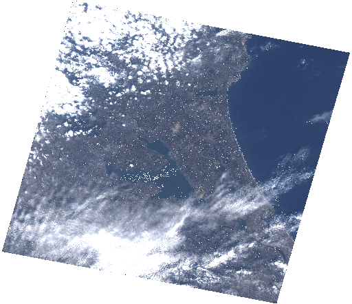
サムネイルを確認してみましょう。
thumbs[0].url()
返り値の URL にブラウザ等でアクセスすると、次の画像が表示されます。
次に、使いやすいように整形された Cloud Optimized GeoTIFF (COG) 形式のファイルを読み込んでみます。
読み込みには GeoTIFF ファイルを xarray.DataArray として読み込むことのできる rioxarray を使用します。
import rioxarray

target_file = next(file for file in files if "webcog" in file["name"])
data = rioxarray.open_rasterio(target_file.url(), masked=True)
pprint.pp(data)
<xarray.DataArray (band: 4, y: 8908, x: 10314)>
[367508448 values with dtype=float32]
Coordinates:
  * band         (band) int64 1 2 3 4
  * x            (x) float64 139.9 139.9 139.9 139.9 ... 140.9 140.9 140.9 140.9
  * y            (y) float64 36.54 36.54 36.54 36.54 ... 35.69 35.69 35.69 35.69
    spatial_ref  int64 0
Attributes:
    AREA_OR_POINT:             Area
    METADATATYPE:              ALOS
    TIFFTAG_IMAGEDESCRIPTION:  03+02+01+04
    scale_factor:              1.0
    add_offset:                0.0
さらに、つくば市の範囲でデータをトリミングします。
clipped_data = data.rio.clip_box(*tsukuba_bbox)
pprint.pp(clipped_data)
<xarray.DataArray (band: 4, y: 3033, x: 1859)>
[22553388 values with dtype=float32]
Coordinates:
  * band         (band) int64 1 2 3 4
  * x            (x) float64 140.0 140.0 140.0 140.0 ... 140.2 140.2 140.2 140.2
  * y            (y) float64 36.24 36.24 36.24 36.24 ... 35.95 35.95 35.95 35.95
    spatial_ref  int64 0
Attributes:
    AREA_OR_POINT:             Area
    METADATATYPE:              ALOS
    TIFFTAG_IMAGEDESCRIPTION:  03+02+01+04
    scale_factor:              1.0
    add_offset:                0.0
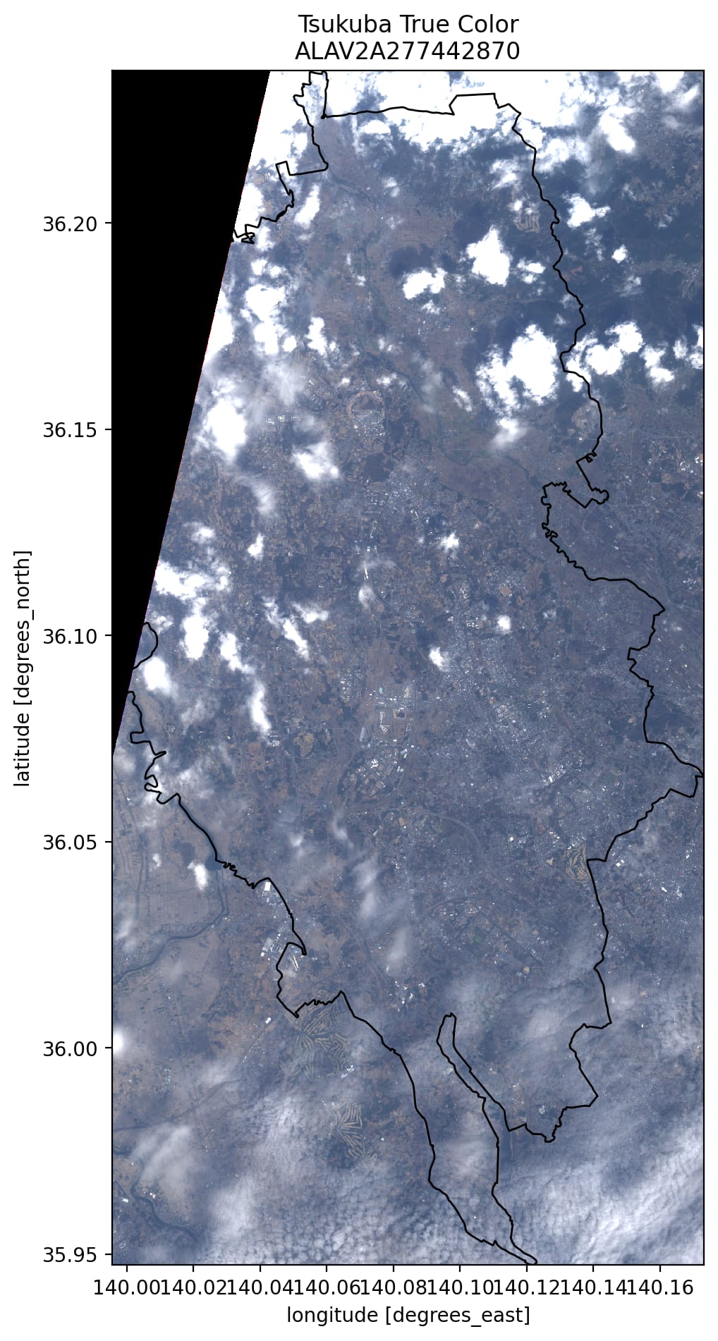
バンド番号1, 2, 3をそれぞれ RGB に割り当て、画像として表示します。
import matplotlib.pyplot as plt

fig, ax = plt.subplots(figsize=(11, 11))
clipped_data.sel(band=[1, 2, 3]).astype('uint8').plot.imshow(ax=ax)
tsukuba_gdf.plot(ax=ax, color="none")
ax.set_title(f"Tsukuba True Color\n{scene['tellus:name']}")
AVNIR-2 には近赤外のバンドもあります。
植物は近赤外を強く反射するため、このバンドを使うことで植生を強調した画像を作ることができます。
R にバンド4(近赤外)、G にバンド1、B にバンド2を割り当てた False Color 画像を表示します。
fig, ax = plt.subplots(figsize=(11, 11))
clipped_data.sel(band=[4, 1, 2]).astype('uint8').plot.imshow(ax=ax)
tsukuba_gdf.plot(ax=ax, color="none")
ax.set_title(f"Tsukuba False Color\n{scene['tellus:name']}")

植生が赤色で強調されていることが確認できます。
参考
Tellus Satellite Data Traveler API の公式チュートリアルは以下にあります。
また、以下の記事では、AVNIR-2 データのより詳しい利用方法が紹介されています。
Discussion