ミニ四駆をモデルとしたGNCシミュレーションの発展的実装
ミニ四駆をモデルとしたGNCシミュレーションの発展的実装:タイヤモデル、制御則の深化[非AIエンジニアによるAI時代のコーディング]
前回の記事「ウェイポイント追従シミュレーションの世界」では、基本的な運動モデルと、ウェイポイント追従のための制御ロジックの構築について解説しました。今回は、さらに一歩進んで、より現実的なシミュレーションを目指し、Vehicleをミニ四駆に当てはめ、以下の点に焦点を当てて掘り下げていきます。今回も、主にCursorのAgent機能を用いて開発しました。
- 高度なタイヤモデルの実装:スリップ率を考慮した摩擦力の計算、回転抵抗、そして旋回時のトルク配分。
- 制御ロジックの洗練:目標速度の動的な調整、最適な進入角度の計算、そしてベジェ曲線を用いた滑らかな軌道生成。
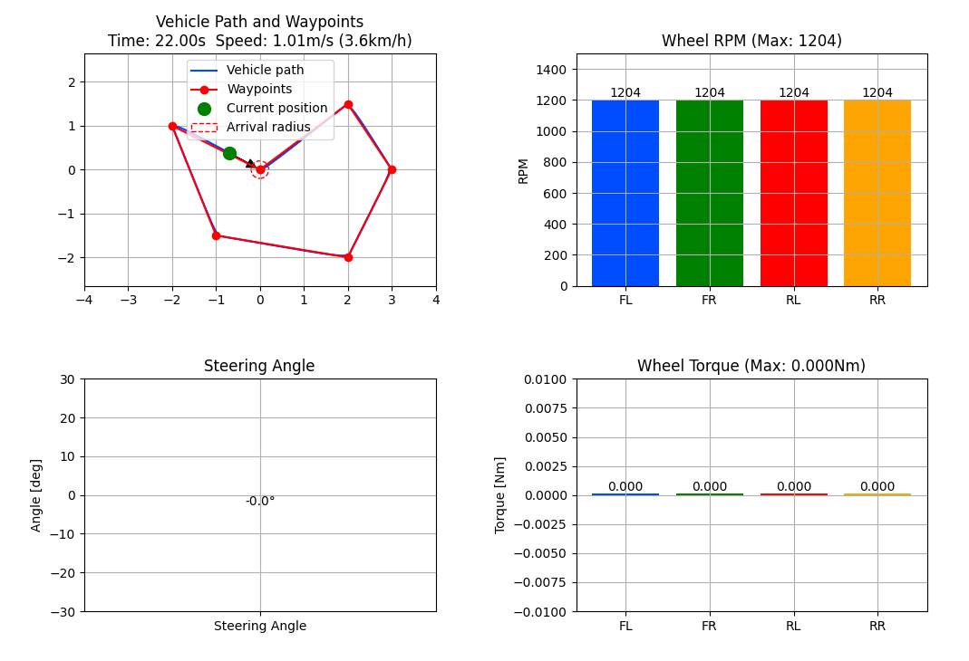
- シミュレーション可視化の強化:タイヤの回転数やトルク、ステアリング角のリアルタイム表示。
1. 高度なタイヤモデルの実装
前回のシミュレーションでは、タイヤの挙動を非常に単純化して扱っていました。しかし、実際のミニ四駆の走行性能をより正確に再現するためには、タイヤのスリップ率とそれによる摩擦力の変化、回転抵抗、そして旋回時の内輪差・外輪差を考慮したトルク配分が不可欠です。
スリップ率を考慮した摩擦力の計算
タイヤのスリップ率は、タイヤの回転速度と車体速度の差によって生じます。スリップ率が大きくなると、タイヤの摩擦力は非線形に変化し、ある点を超えると減少します。この現象をシミュレーションするために、「マジックフォーミュラ」と呼ばれるタイヤモデルを簡略化した形で実装しました。
def calculate_slip_ratio(self, wheel_angular_velocity, vehicle_speed):
    """スリップ率の計算"""
    wheel_speed = wheel_angular_velocity * self.wheel_radius
    if abs(vehicle_speed) < 0.1:  # 低速時のゼロ除算防止
        return 0.0
    return (wheel_speed - vehicle_speed) / max(abs(vehicle_speed), 0.1)

def calculate_wheel_force(self, slip_ratio):
    """タイヤの発生力を計算(簡略化したマジックフォーミュラ)"""
    B = 10.0  # スティフネスファクター
    C = 1.9  # 形状ファクター
    D = self.normal_force * self.friction_coefficient  # 最大力

    return D * np.sin(C * np.arctan(B * slip_ratio))
回転抵抗の考慮
ミニ四駆の走行において、モーターやギヤなどの回転機構による抵抗は無視できません。特に、低速域ではこの抵抗が運動に大きな影響を与えます。そこで、タイヤの角速度に比例する回転抵抗をモデルに組み込みました。
# 車両クラスの初期化時に回転抵抗係数を設定
self.resistance_coefficient = 1e-5  # 回転抵抗係数 [Nm/(rad/s)]

def update_wheel_state(self, wheel_id, torque, dt):
    """個々のタイヤの状態を更新(地面との摩擦を考慮)"""
    wheel = self.wheels[wheel_id]

    # 回転抵抗を考慮
    resistance_torque = -wheel['angular_velocity'] * self.resistance_coefficient

    # 地面との摩擦によるトルクを計算
    ground_friction_coeff = 0.8  # 地面との摩擦係数
    normal_force = (self.vehicle_mass * 9.81) / 4  # 各車輪にかかる垂直抗力
    ground_friction_torque = ground_friction_coeff * normal_force * self.wheel_radius

    # タイヤの周速と車体速度の差からスリップ率を計算
    wheel_speed = wheel['angular_velocity'] * self.wheel_radius
    slip_ratio = self.calculate_slip_ratio(wheel['angular_velocity'], self.v)

    # スリップ率に基づく摩擦力を計算
    friction_force = self.calculate_wheel_force(slip_ratio)
    friction_torque = friction_force * self.wheel_radius

    # 合計トルクの計算
    net_torque = torque + resistance_torque + friction_torque

    # 減速時の特別処理
    if torque < 0 and self.v > 0.1:
        # 急激な回転数の低下を防ぐ
        deceleration_factor = np.clip(abs(self.v) / 2.0, 0.1, 1.0)
        net_torque = net_torque * deceleration_factor

    # 角加速度の計算と角速度の更新
    angular_acceleration = net_torque / self.wheel_inertia
    new_angular_velocity = wheel['angular_velocity'] + angular_acceleration * dt

    # 車体が動いている場合、タイヤの最小回転速度を維持
    if abs(self.v) > 0.1:
        min_angular_velocity = (self.v * 0.9) / self.wheel_radius  # 10%のスリップを許容
        new_angular_velocity = max(new_angular_velocity, min_angular_velocity)

    wheel['angular_velocity'] = new_angular_velocity
    wheel['rpm'] = new_angular_velocity * 60 / (2 * np.pi)
    wheel['slip_ratio'] = slip_ratio
    wheel['torque'] = torque
旋回時のトルク配分
旋回時には、内輪と外輪で走行距離が異なるため、それぞれのタイヤに適切なトルクを配分する必要があります。これを考慮することで、よりスムーズで効率的な旋回をシミュレーションできます。
def update(self, v, omega, dt):
    """車両の状態を更新"""
    # 加速度の計算
    self.acceleration = (v - self.v) / dt

    # ステアリング角の計算と制限
    if abs(omega) > 1e-6:
        turning_radius = abs(v / omega)
        self.steering_angle = np.arctan(self.wheelbase / turning_radius)
        if omega < 0:
            self.steering_angle = -self.steering_angle
    else:
        self.steering_angle = 0.0

    self.steering_angle = np.clip(self.steering_angle,
                                -self.max_steering_angle,
                                self.max_steering_angle)

    # 各タイヤのトルク計算(簡略化したモデル)
    base_torque = self.acceleration * self.wheel_radius * (self.vehicle_mass / 4)

    # 旋回時の荷重移動を考慮したトルク配分
    if abs(self.steering_angle) > 1e-6:
        turning_radius = self.wheelbase / np.tan(abs(self.steering_angle))
        inner_ratio = (turning_radius - (self.track_width / 2)) / turning_radius
        outer_ratio = (turning_radius + (self.track_width / 2)) / turning_radius

        # ... (トルク配分計算)
    else:
        # 直進時は均等配分
        torques = {wheel: base_torque for wheel in self.wheels.keys()}

    # 各タイヤの状態更新
    for wheel_id, torque in torques.items():
        self.update_wheel_state(wheel_id, torque, dt)

    # 位置と姿勢の更新
    self.x += self.v * np.cos(self.theta) * dt
    self.y += self.v * np.sin(self.theta) * dt
    self.theta += omega * dt
    self.v = v
    self.omega = omega
    self.prev_v = v
    self.prev_omega = omega
2. 制御ロジックの洗練
より複雑な走行シナリオに対応するために、制御ロジックにも磨きをかけました。
目標速度の動的な調整
前回のシミュレーションでは、目標速度を一定としていましたが、今回は、カーブの曲率や目標地点までの距離に応じて動的に速度を調整するようにしました。これにより、カーブでは減速し、直線では加速するなど、より自然な走行が可能になりました。
def calc_target_velocity(current_waypoint, next_waypoint, vehicle_pos,
                        max_velocity=1.0, min_velocity=0.2, look_ahead_factor=0.5):
    # 現在のウェイポイントまでの距離
    dist_to_current = np.linalg.norm(current_waypoint - vehicle_pos)

    # 現在のウェイポイントから次のウェイポイントへのベクトル
    next_vector = next_waypoint - current_waypoint
    next_distance = np.linalg.norm(next_vector)
    next_direction = next_vector / next_distance if next_distance > 0 else np.array([0, 0])

    # 現在のウェイポイントへの方向ベクトル
    current_vector = current_waypoint - vehicle_pos
    current_direction = current_vector / np.linalg.norm(current_vector) if dist_to_current > 0 else np.array([0, 0])

    # 方向変化の計算
    direction_change = np.dot(current_direction, next_direction)
    direction_change = np.clip(direction_change, -1, 1)  # 数値誤差対策
    turn_angle = np.arccos(direction_change)

    # 曲率に基づく速度調整
    turn_factor = np.cos(turn_angle)  # 方向変化が大きいほど小さくなる

    # 距離に基づく速度調整
    distance_factor = np.clip(dist_to_current / (next_distance * look_ahead_factor), 0, 1)

    # 目標速度の計算
    target_velocity = max_velocity * turn_factor * (0.5 + 0.5 * distance_factor)
    target_velocity = np.clip(target_velocity, min_velocity, max_velocity)

    return target_velocity
最適な進入角度の計算
次のウェイポイントへの進入角度を考慮することで、よりスムーズなコーナリングを実現しました。
def calc_optimal_approach(current_pos, current_waypoint, next_waypoint):
    if next_waypoint is None:
        return 0.6, atan2(current_waypoint[1] - current_pos[1],
                         current_waypoint[0] - current_pos[0])

    # 現在のウェイポイントまでのベクトル
    current_vector = current_waypoint - current_pos
    current_distance = np.linalg.norm(current_vector)

    # 次のウェイポイントへのベクトル
    next_vector = next_waypoint - current_waypoint
    next_distance = np.linalg.norm(next_vector)

    # 方向変化の計算
    if current_distance > 0.1:
        current_direction = current_vector / current_distance
        next_direction = next_vector / next_distance
        direction_change = np.arccos(np.clip(np.dot(current_direction, next_direction), -1.0, 1.0))

        # 進入角と進出角を計算
        entry_angle = atan2(current_vector[1], current_vector[0])
        exit_angle = atan2(next_vector[1], next_vector[0])
        angle_diff = abs((exit_angle - entry_angle + 3*pi) % (2*pi) - pi)
    else:
        direction_change = 0.0
        angle_diff = 0.0

    # 基本速度を設定
    base_speed = 1.2

    # 方向変化に基づく速度調整
    if direction_change > pi/2:
        speed_factor = 0.5
    else:
        # 進入角と進出角の差に基づく速度調整
        speed_factor = np.clip(1.0 - angle_diff/pi, 0.5, 0.9)

    # 最終的な速度を決定
    optimal_speed = base_speed * speed_factor
    optimal_speed = max(0.5, optimal_speed)

    # 進入角の計算(バランスを考慮)
    if direction_change > pi/2:
        blend_factor = 0.3
    else:
        # 角度差に基づくブレンド係数
        blend_factor = 0.3 + 0.2 * (1.0 - angle_diff/pi)

    target_x = current_waypoint[0] + blend_factor * (next_waypoint[0] - current_waypoint[0])
    target_y = current_waypoint[1] + blend_factor * (next_waypoint[1] - current_waypoint[1])

    optimal_angle = atan2(target_y - current_pos[1],
                         target_x - current_pos[0])

    return optimal_speed, optimal_angle
ベジェ曲線を用いた滑らかな軌道生成
ウェイポイントを直線で結ぶのではなく、ベジェ曲線を用いて滑らかな軌道を生成することで、より自然な走行をシミュレーションしました。
def calc_intermediate_target(current_pos, current_waypoint, next_waypoint, radius=1.0):
    if next_waypoint is None:
        return current_waypoint

    # 現在のウェイポイントまでのベクトル
    current_vector = current_waypoint - current_pos
    current_distance = np.linalg.norm(current_vector)

    # 次のウェイポイントへのベクトル
    next_vector = next_waypoint - current_waypoint
    next_distance = np.linalg.norm(next_vector)

    # 単位ベクトルの計算
    if current_distance > 0.1 and next_distance > 0.1:
        current_direction = current_vector / current_distance
        next_direction = next_vector / next_distance

        # 進行方向の変化角度を計算
        direction_change = np.arccos(np.clip(np.dot(current_direction, next_direction), -1.0, 1.0))

        # ベジェ曲線のための制御点を計算
        if direction_change > pi/6:  # 30度以上の方向変化で曲線を生成
            # 曲線の大きさを角度に応じて調整
            curve_scale = np.clip(direction_change / pi, 0.3, 0.8)

            # 現在の進行方向に沿った制御点
            control_point1 = current_waypoint - current_direction * (next_distance * curve_scale)

            # 次の進行方向に沿った制御点
            control_point2 = current_waypoint + next_direction * (current_distance * curve_scale)

            # 現在位置からの進行距離に応じてベジェ曲線上の点を計算
            t = np.clip(current_distance / (current_distance + next_distance), 0.0, 1.0)

            # 3次ベジェ曲線の計算
            intermediate_target = (1-t)**3 * current_pos + \
                                3*(1-t)**2*t * control_point1 + \
                                3*(1-t)*t**2 * control_point2 + \
                                t**3 * next_waypoint

            print(f"\nBezier Curve Debug:")
            print(f"Direction change: {degrees(direction_change):.1f}°")
            print(f"Curve scale: {curve_scale:.3f}")
            print(f"Bezier parameter t: {t:.3f}")

            return intermediate_target

    return current_waypoint
3. シミュレーション可視化の強化
シミュレーション結果をより分かりやすくするために、以下のような可視化機能を強化しました。
- タイヤの回転数とトルクの表示:各タイヤの回転数(RPM)とトルクをリアルタイムでグラフ表示。
- ステアリング角の表示:ステアリング角を数値とグラフで表示。
これらの可視化機能により、シミュレーション中のミニ四駆の挙動をより詳細に把握できるようになりました。
シミュレーション結果
出力した様子です。
まとめ
今回の記事では、ミニ四駆としてシミュレーションをさらに進化させるために、高度なタイヤモデルの実装、制御ロジックの洗練、そしてシミュレーション可視化の強化について解説しました。これらの改良により、シミュレーションの精度が向上し、より現実的なミニ四駆の走行を再現できるようになりました。
しかし、たかがミニ四駆と言っても世界は奥深く、まだまだ探求すべき課題はたくさんあります。今後の展望としては、サスペンションモデルの導入、コースレイアウトの最適化、そして強化学習を用いたより高度な制御アルゴリズムの開発などが考えられます。
今回もAIによるコーディングのみで開発しましたが、実際に物理則を検索させ、実装させるという応用的な使い方も十分に可能でした。パラメータの調整など、AIがコーディングしたものの内容を理解して指示を出せば、十分に活用していける環境を構築できるものと考えます。
AIによるコーディングには、途轍も無い可能性を感じますね。
Discussion