ウェイポイント追従シミュレーションの世界

ウェイポイント追従シミュレーションの世界[非AIエンジニアによるAI時代のコーディング]

はじめに：AIとロボット制御の未来を切り拓く

皆さん、こんにちは！この記事では、「非AIエンジニアによるAI時代のコーディング」シリーズとして、Pythonを使った基本的なロボット制御をコーディングします。特に、ロボットが指定された経路を自動で辿る「ウェイポイント追従」という技術に焦点を当て、そのシミュレーションを実際にPythonで実装してみました。開発においては、CursorのAgent機能を主に用いました。

今回のプロダクト：2次元ウェイポイント追従シミュレーション

今回開発するのは、2次元平面上を移動するロボットが、あらかじめ設定されたウェイポイント（経由地点）を順番に辿っていくシミュレーションプログラムです。

このプログラムを使うことで、

• ロボットがどのように目標地点に向かって動くのか
• どのようなアルゴリズムで制御すれば、正確に経路を追従できるのか

といった、ロボット制御の基本的な考え方を再現することができます。

シミュレーション結果は、グラフで可視化されるので、動きを目で見て確認できるのも面白いところです。

開発の背景：AIが拓くロボット制御の可能性

近年、AI技術の発展は目覚ましく、ロボット制御の分野にも大きな変化をもたらしています。

例えば、

• 強化学習: ロボット自身が試行錯誤を繰り返しながら、最適な制御方法を学習する
• 深層学習: カメラなどのセンサー情報から、周囲の状況を認識し、より複雑なタスクを実行する

といった技術が、実用化され始めています。

この記事で紹介するウェイポイント追従は、これらの高度なAI技術を活用した制御の基礎となる重要な技術です。

プログラム解説：Pythonでロボットを動かしてみよう！

それでは、実際にPythonで書かれたプログラムを見ていきましょう。

プログラム全体構成

このプログラムは、大きく分けて以下の要素で構成されています。

1. Vehicleクラス: ロボットの状態（位置、角度、速度など）を管理する
2. 制御アルゴリズム: ロボットを目標地点に導くための計算を行う関数群
3. シミュレーション: ロボットの動きを時間経過とともに計算し、結果をグラフで表示する

Vehicleクラス

まずは、ロボットの状態を管理するVehicleクラスを見てみましょう。

class Vehicle:
    def __init__(self, x=0.0, y=0.0, theta=0.0, v=0.0, omega=0.0):
        self.x = x
        self.y = y
        self.theta = theta
        self.v = v
        self.omega = omega
        self.prev_v = v
        self.prev_omega = omega
        self.max_v = 1.0      # 最大速度
        self.max_omega = 1.0  # 最大角速度
        self.prev_dist_error = 0.0  # 距離誤差の前回値
        self.prev_angle_error = 0.0  # 角度誤差の前回値
        self.waypoint_reach_count = 0  # 到達判定のカウンタを追加
        self.reach_threshold_dist = 0.2  # 到達判定の距離閾値
        self.reach_threshold_vel = 0.5  # 到達判定の速度閾値を緩和
        self.reach_count_required = 3   # 必要な到達判定回数を減少
        # 積分項用の変数を追加
        self.sum_dist_error = 0.0
        self.sum_angle_error = 0.0
        self.max_sum_dist_error = 1.0   # 5.0から1.0に減少
        self.max_sum_angle_error = 0.5  # 2.0から0.5に減少
        # 車両の物理パラメータを追加
        self.wheel_base = 0.5     # ホイールベース[m]
        self.min_turn_radius = 0.6  # 最小回転半径[m]
        self.max_steering_angle = pi/4  # 最大ステアリング角[rad]

    def update(self, v, omega, dt):
        self.x += self.v * np.cos(self.theta) * dt
        self.y += self.v * np.sin(self.theta) * dt
        self.theta += self.omega * dt
        self.v = v
        self.omega = omega
        self.prev_v = v
        self.prev_omega = omega

このクラスは、ロボットの位置（x、y）、進行方向の角度（theta）、速度（v）、角速度（omega）などの情報を保持します。

制御アルゴリズム

ロボットを目標地点に導くための制御アルゴリズムは、いくつかの関数に分かれています。

1. calc_target_velocity: 次のウェイポイントを考慮して、最適な目標速度を計算する
2. calc_optimal_rotation_direction: 現在の進行方向と目標地点の方向から、最適な回転方向を決定する
3. calc_control_input: PID制御を用いて、ロボットへの制御入力（速度と角速度）を計算する
   これらの関数が連携することで、ロボットはスムーズにウェイポイントを追従することができます。

def calc_control_input(vehicle, target_x, target_y, dt, next_waypoint=None,
                      Kp_v=1.2, Ki_v=0.1, Kd_v=0.4,
                      Kp_omega=2.0, Ki_omega=0.05, Kd_omega=0.1,
                      max_v_rate=1.0, max_omega_rate=1.0,
                      alpha=0.8):
    """
    目標地点に向かうためのPID制御入力を計算（到達優先版）
    """
    current_pos = np.array([vehicle.x, vehicle.y])
    current_waypoint = np.array([target_x, target_y])
    
    # 物理パラメータ
    MAX_ACCELERATION = 0.5  # m/s^2
    MAX_DECELERATION = 0.8  # m/s^2
    MIN_VELOCITY = 0.2      # m/s
    MAX_VELOCITY = 1.2      # m/s
    
    # 実際のwaypointまでの直接距離を計算
    direct_distance = np.linalg.norm(current_waypoint - current_pos)
    
    # 到達判定の閾値を小さく設定
    arrival_threshold = 0.2
    
    # デバッグ情報
    print(f"\nWaypoint Approach Debug:")
    print(f"Current position: ({vehicle.x:.3f}, {vehicle.y:.3f})")
    print(f"Target waypoint: ({target_x:.3f}, {target_y:.3f})")
    print(f"Direct distance: {direct_distance:.3f}m")
    print(f"Current velocity: {vehicle.v:.3f}m/s")
    
    # 到達判定（より厳密に）
    if direct_distance <= arrival_threshold:
        print(f"Waypoint reached: distance={direct_distance:.3f}m")
        if next_waypoint is None:
            return 0.0, 0.0, True
        else:
            next_waypoint = np.array(next_waypoint)
            target_theta = atan2(next_waypoint[1] - vehicle.y,
                               next_waypoint[0] - vehicle.x)
            angle_error = calc_optimal_rotation_direction(vehicle.theta, target_theta, vehicle.v)
            return MIN_VELOCITY, Kp_omega * angle_error, True
    
    # waypointへの直接アプローチを優先
    target_theta = atan2(current_waypoint[1] - vehicle.y,
                        current_waypoint[0] - vehicle.x)
    angle_error = calc_optimal_rotation_direction(vehicle.theta, target_theta, vehicle.v)
    
    # 角度誤差が大きい場合は、その場で回転
    if abs(angle_error) > pi/4:  # 45度以上の角度誤差
        print("Large angle error - rotating in place")
        return MIN_VELOCITY * 0.5, Kp_omega * angle_error * 1.5, False
    
    # 目標速度の計算（距離に応じて）
    if direct_distance < arrival_threshold * 2.0:
        # 近距離では低速
        target_v = MIN_VELOCITY
    else:
        # 距離に応じた速度設定
        target_v = min(
            MIN_VELOCITY + (MAX_VELOCITY - MIN_VELOCITY) * (direct_distance / (arrival_threshold * 5.0)),
            MAX_VELOCITY
        )
    
    # 角度誤差に応じた速度調整
    speed_factor = np.cos(angle_error)  # 角度誤差が大きいほど速度を下げる
    target_v *= max(0.3, speed_factor)
    
    # 加速度制限に基づく速度変化の計算
    v_error = target_v - vehicle.v
    if v_error > 0:
        # 加速時
        max_dv = MAX_ACCELERATION * dt
        v = min(vehicle.v + max_dv, target_v)
    else:
        # 減速時
        max_dv = MAX_DECELERATION * dt
        v = max(vehicle.v - max_dv, target_v)
    
    # 最終的な速度の制限
    v = np.clip(v, MIN_VELOCITY * 0.5, MAX_VELOCITY)
    
    # 角速度の計算（より積極的な方向修正）
    omega = Kp_omega * angle_error * 1.2
    omega = np.clip(omega, -max_omega_rate, max_omega_rate)
    
    # 速度の平滑化（急激な変化を防ぐ）
    if hasattr(vehicle, 'prev_v'):
        v = 0.7 * v + 0.3 * vehicle.prev_v
    vehicle.prev_v = v
    
    # デバッグ情報
    print(f"Target velocity: {target_v:.3f}m/s")
    print(f"Applied velocity: {v:.3f}m/s")
    print(f"Angle error: {degrees(angle_error):.1f}°")
    
    return v, omega, False

プログラム詳細解説

ここまでで、Vehicleクラスと、ロボットを制御するための主要な関数calc_control_inputについて解説しました。続いて、残りの重要な関数について、さらに詳しく見ていきましょう。

calc_target_velocity関数：最適な目標速度を計算する

def calc_target_velocity(current_waypoint, next_waypoint, vehicle_pos, 
                        max_velocity=1.0, min_velocity=0.2, look_ahead_factor=0.5):
    """
    次のウェイポイントを考慮した目標速度を計算
    
    Args:
        current_waypoint: 現在の目標ウェイポイント
        next_waypoint: 次のウェイポイント
        vehicle_pos: 車両の現在位置 [x, y]
        max_velocity: 最大速度
        min_velocity: 最小速度
        look_ahead_factor: 先読み係数
    """
    if next_waypoint is None:
        # 最終ウェイポイントの場合は減速
        return min_velocity
    
    # 現在のウェイポイントまでの距離
    dist_to_current = np.linalg.norm(current_waypoint - vehicle_pos)
    
    # 現在のウェイポイントから次のウェイポイントへのベクトル
    next_vector = next_waypoint - current_waypoint
    next_distance = np.linalg.norm(next_vector)
    next_direction = next_vector / next_distance if next_distance > 0 else np.array([0, 0])
    
    # 現在のウェイポイントへの方向ベクトル
    current_vector = current_waypoint - vehicle_pos
    current_direction = current_vector / np.linalg.norm(current_vector) if dist_to_current > 0 else np.array([0, 0])
    
    # 方向変化の計算
    direction_change = np.dot(current_direction, next_direction)
    direction_change = np.clip(direction_change, -1, 1)  # 数値誤差対策
    turn_angle = np.arccos(direction_change)
    
    # 曲率に基づく速度調整
    turn_factor = np.cos(turn_angle)  # 方向変化が大きいほど小さくなる
    
    # 距離に基づく速度調整
    distance_factor = np.clip(dist_to_current / (next_distance * look_ahead_factor), 0, 1)
    
    # 目標速度の計算
    target_velocity = max_velocity * turn_factor * (0.5 + 0.5 * distance_factor)
    target_velocity = np.clip(target_velocity, min_velocity, max_velocity)
    
    return target_velocity

この関数は、ロボットが次のウェイポイントにスムーズに到達するために、最適な目標速度を計算します。

• なぜ必要か: ロボットは、ただウェイポイントに向かえば良いわけではありません。カーブの手前では減速したり、次のウェイポイントが遠い場合は加速するなど、状況に応じて速度を調整する必要があります。calc_target_velocity関数は、これらの判断を自動で行います。
• 設定理由:
  max_velocity、min_velocity: ロボットの物理的な制限に基づく速度範囲。
  look_ahead_factor: 次のウェイポイントをどれだけ「先読み」して速度を調整するかを決める係数。この値を調整することで、ロボットの滑らかな動きを実現します。

calc_optimal_rotation_direction関数：最適な回転方向を決定する

def calc_optimal_rotation_direction(current_angle, target_angle, current_speed):
    """
    現在の進行方向と速度を考慮した最適な回転方向の決定
    """
    # 基本の角度差を計算（-πからπの範囲に正規化）
    angle_diff = (target_angle - current_angle + pi) % (2*pi) - pi
    
    # 速度が十分にある場合のみ方向転換を制限
    if abs(current_speed) > 0.1:
        # 大きな方向転換が必要な場合は徐々に曲がる
        if abs(angle_diff) > pi/2:
            return np.sign(angle_diff) * pi/2
    
    return angle_diff

この関数は、ロボットが目標角度に向かって効率的に回転するために、最適な回転方向と回転量を計算します。

• なぜ必要か: ロボットは、目標地点の方向に常に真っ直ぐ向かえるとは限りません。特に、速度が出ている状態で急な方向転換をすると、大きく膨らんでしまいます。calc_optimal_rotation_direction関数は、現在の速度と目標角度を考慮して、滑らかな回転を実現します。
• 設定理由:
  速度が遅い場合は、その場での回転を許可し、素早く方向転換できるようにします。
  速度が速い場合は、緩やかな回転を促し、安定性を確保します。

calc_optimal_approach関数：最適な進入方法を計算する

def calc_optimal_approach(current_pos, current_waypoint, next_waypoint):
    """
    次のウェイポイントへの最適な進入角と速度を計算（バランス改善版）
    """
    if next_waypoint is None:
        return 0.6, atan2(current_waypoint[1] - current_pos[1],
                         current_waypoint[0] - current_pos[0])
    
    # 現在のウェイポイントまでのベクトル
    current_vector = current_waypoint - current_pos
    current_distance = np.linalg.norm(current_vector)
    
    # 次のウェイポイントへのベクトル
    next_vector = next_waypoint - current_waypoint
    next_distance = np.linalg.norm(next_vector)
    
    # 方向変化の計算
    if current_distance > 0.1:
        current_direction = current_vector / current_distance
        next_direction = next_vector / next_distance
        direction_change = np.arccos(np.clip(np.dot(current_direction, next_direction), -1.0, 1.0))
        
        # 進入角と進出角を計算
        entry_angle = atan2(current_vector[1], current_vector[0])
        exit_angle = atan2(next_vector[1], next_vector[0])
        angle_diff = abs((exit_angle - entry_angle + 3*pi) % (2*pi) - pi)
    else:
        direction_change = 0.0
        angle_diff = 0.0
    
    # 基本速度を設定
    base_speed = 1.2
    
    # 方向変化に基づく速度調整
    if direction_change > pi/2:
        speed_factor = 0.5
    else:
        # 進入角と進出角の差に基づく速度調整
        speed_factor = np.clip(1.0 - angle_diff/pi, 0.5, 0.9)
    
    # 最終的な速度を決定
    optimal_speed = base_speed * speed_factor
    optimal_speed = max(0.5, optimal_speed)
    
    # 進入角の計算（バランスを考慮）
    if direction_change > pi/2:
        blend_factor = 0.3
    else:
        # 角度差に基づくブレンド係数
        blend_factor = 0.3 + 0.2 * (1.0 - angle_diff/pi)
    
    target_x = current_waypoint[0] + blend_factor * (next_waypoint[0] - current_waypoint[0])
    target_y = current_waypoint[1] + blend_factor * (next_waypoint[1] - current_waypoint[1])
    
    optimal_angle = atan2(target_y - current_pos[1],
                         target_x - current_pos[0])
    
    return optimal_speed, optimal_angle

この関数は、ロボットが次のウェイポイントにどのように進入するかを計算します。

• なぜ必要か: ロボットがカクカクと動くのではなく、滑らかにウェイポイントを通過するためには、進入角度と速度を適切に制御する必要があります。calc_optimal_approach関数は、これらの要素を考慮して、より自然な動きを実現します。
• 設定理由:
  次のウェイポイントとの角度に応じて速度を調整し、急カーブでは減速するようにします。
  進入角度を調整することで、ウェイポイントをスムーズに通過できるようにします。

calc_intermediate_target関数：まわり込み軌道のための中間目標点を計算する

def calc_intermediate_target(current_pos, current_waypoint, next_waypoint, radius=1.0):
    """
    まわり込み軌道のための中間目標点を計算（滑らか化版）
    """
    if next_waypoint is None:
        return current_waypoint
    
    # 現在のウェイポイントまでのベクトル
    current_vector = current_waypoint - current_pos
    current_distance = np.linalg.norm(current_vector)
    
    # 次のウェイポイントへのベクトル
    next_vector = next_waypoint - current_waypoint
    next_distance = np.linalg.norm(next_vector)
    
    # 単位ベクトルの計算
    if current_distance > 0.1 and next_distance > 0.1:
        current_direction = current_vector / current_distance
        next_direction = next_vector / next_distance
        
        # 進行方向の変化角度を計算
        direction_change = np.arccos(np.clip(np.dot(current_direction, next_direction), -1.0, 1.0))
        
        # ベジェ曲線のための制御点を計算
        if direction_change > pi/6:  # 30度以上の方向変化で曲線を生成
            # 曲線の大きさを角度に応じて調整
            curve_scale = np.clip(direction_change / pi, 0.3, 0.8)
            
            # 現在の進行方向に沿った制御点
            control_point1 = current_waypoint - current_direction * (next_distance * curve_scale)
            
            # 次の進行方向に沿った制御点
            control_point2 = current_waypoint + next_direction * (current_distance * curve_scale)
            
            # 現在位置からの進行距離に応じてベジェ曲線上の点を計算
            t = np.clip(current_distance / (current_distance + next_distance), 0.0, 1.0)
            
            # 3次ベジェ曲線の計算
            intermediate_target = (1-t)**3 * current_pos + \
                                3*(1-t)**2*t * control_point1 + \
                                3*(1-t)*t**2 * control_point2 + \
                                t**3 * next_waypoint
            
            print(f"\nBezier Curve Debug:")
            print(f"Direction change: {degrees(direction_change):.1f}°")
            print(f"Curve scale: {curve_scale:.3f}")
            print(f"Bezier parameter t: {t:.3f}")
            
            return intermediate_target
    
    return current_waypoint

この関数は、ロボットがウェイポイントを通過する際に、より滑らかな軌道を描くための中間目標点を計算します。

• なぜ必要か: ウェイポイントを直線的に結ぶだけでは、ロボットの動きが不自然になる場合があります。calc_intermediate_target関数は、ベジェ曲線という数学的な手法を使って、より自然な「まわり込み軌道」を生成します。
• 設定理由:
  ベジェ曲線の制御点を、現在のウェイポイントと次のウェイポイントの位置関係から自動的に計算します。
  radiusパラメータで、まわり込み軌道の大きさを調整できます。

is_waypoint_reached関数：ウェイポイントへの到達判定を行う

def is_waypoint_reached(vehicle, current_waypoint, prev_waypoint, 
                       circle_diameter=0.5, vel_threshold=0.5):
    """
    ウェイポイントへの到達判定（改善版）
    """
    # 距離による判定
    dist_to_waypoint = sqrt((current_waypoint[0] - vehicle.x)**2 + 
                           (current_waypoint[1] - vehicle.y)**2)
    
    # 速度の大きさを計算
    velocity_magnitude = sqrt(vehicle.v**2 + (vehicle.omega * vehicle.wheel_base)**2)
    
    # デバッグ情報を出力
    print(f"\nWaypoint Reach Check:")
    print(f"Distance to waypoint: {dist_to_waypoint:.3f}m (threshold: {circle_diameter/2:.3f}m)")
    print(f"Velocity magnitude: {velocity_magnitude:.3f}m/s (threshold: {vel_threshold:.3f}m/s)")
    print(f"Current reach count: {vehicle.waypoint_reach_count}/{vehicle.reach_count_required}")
    
    # 到達判定（速度条件を緩和）
    reached = (dist_to_waypoint < circle_diameter/2 and 
              velocity_magnitude < vel_threshold)
    
    if reached:
        print("✓ Waypoint reach conditions met")
    else:
        if dist_to_waypoint >= circle_diameter/2:
            print("✗ Distance condition not met")
        if velocity_magnitude >= vel_threshold:
            print("✗ Velocity condition not met")
    
    return reached

この関数は、ロボットがウェイポイントに十分に近づいたかどうかを判定します。

• なぜ必要か: シミュレーションでは、ロボットが完全にウェイポイント上に静止することは稀です。ある程度の誤差を許容して、「十分に近づいた」と判断する必要があります。is_waypoint_reached関数は、そのための基準を提供します。
• 設定理由:
  circle_diameter: ウェイポイントを中心とした到達判定円の直径。
  vel_threshold: ウェイポイント到達時に、ロボットの速度が十分に遅いことを確認するための閾値。

シミュレーション

最後に、シミュレーション部分では、ロボットの状態を時間経過とともに更新し、その結果をグラフで表示します。

def main():
    # プログラム開始時に既存のプロットをクリア
    plt.close('all')
    
    # 日本の航空路ウェイポイント
    waypoints = np.array([
        [0.0, 0.0],       # RJTT (東京/羽田) を原点として
        [2.0, 1.5],       # ADDUM (関東の北東)
        [3.0, 0.0],       # GODIN (太平洋上)
        [2.0, -2.0],      # SMILE (伊豆半島沖)
        [-1.0, -1.5],     # MIURA (三浦半島沖)
        [-2.0, 1.0],      # KAGNA (東京湾北部)
        [0.0, 0.0]        # RJTT (東京/羽田) に戻る
    ])

    # 初期位置と姿勢
    vehicle = Vehicle(x=0.0, y=0.0, theta=0.0, v=0.0)
    
    # シミュレーションパラメータ
    dt = 0.1
    time = 0.0
    max_simulation_time = 100.0
    
    # 結果保存用の配列
    times = []
    x = []
    y = []
    
    # 現在のウェイポイントのインデックス
    current_wp_index = 1
    
    # メインループ内のプロット処理
    plt.ion()  # インタラクティブモードをオン
    fig = plt.figure(figsize=(8, 8))

    while time < max_simulation_time and current_wp_index < len(waypoints):
        # 現在のウェイポイント
        current_waypoint = waypoints[current_wp_index]
        
        # 次のウェイポイント（最後のウェイポイントの場合はNone）
        next_waypoint = waypoints[current_wp_index + 1] if current_wp_index + 1 < len(waypoints) else None
        
        # 制御入力の計算
        v, omega, reached = calc_control_input(
            vehicle,
            current_waypoint[0],
            current_waypoint[1],
            dt,
            next_waypoint
        )
        
        # 車両の状態を更新
        vehicle.update(v, omega, dt)
        
        # 結果の保存
        times.append(time)
        x.append(vehicle.x)
        y.append(vehicle.y)
        
        # ウェイポイントに到達したら次のウェイポイントへ
        if reached:
            print(f"\nReached waypoint {current_wp_index}: ({current_waypoint[0]:.2f}, {current_waypoint[1]:.2f})")
            current_wp_index += 1
        
        # リアルタイムプロット
        plt.clf()  # 前回のプロットをクリア
        plt.plot(x, y, 'b-', label='Vehicle path')
        plt.plot(waypoints[:,0], waypoints[:,1], 'ro-', label='Waypoints')
        plt.plot(vehicle.x, vehicle.y, 'go', markersize=10, label='Current position')
        
        # 現在のウェイポイントの到達目標半径を表示
        arrival_threshold = 0.2  # 到達判定の閾値
        circle = plt.Circle((current_waypoint[0], current_waypoint[1]), arrival_threshold, 
                           color='r', fill=False, linestyle='--', label='Arrival radius')
        plt.gca().add_patch(circle)
        
        plt.axis('equal')
        plt.grid(True)
        plt.legend()
        plt.title(f'Vehicle Path and Waypoints (Time: {time:.1f}s)')
        plt.xlim(-4.0, 4.0)
        plt.ylim(-4.0, 4.0)
        plt.draw()
        plt.pause(0.001)
        
        time += dt
    
    # シミュレーション終了後、最終プロットを保持
    plt.ioff()
    plt.show()

matplotlibというライブラリを使うことで、ロボットの軌跡やウェイポイントを視覚的に確認することができます。

シミュレーション結果：ロボットの動きを可視化する

プログラムを実行すると、以下のようなグラフが表示されます。

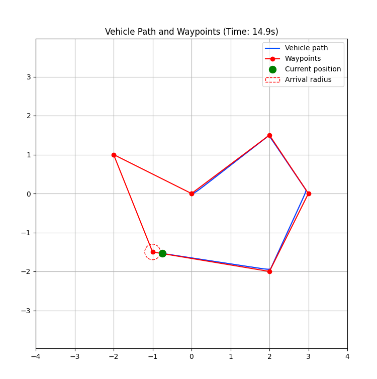
このグラフは、2次元平面上でのロボットの動きを示しています。

• 青線 (Vehicle path): ロボットが実際に辿った経路
• 赤丸 (Waypoints): ロボットが目指す経由地点
• 緑丸 (Current position): 現在のロボットの位置
• 赤点線円 (Arrival radius): ウェイポイントへの到達判定に使用する円

このグラフを見ることで、ロボットがどのようにウェイポイントを追従しているのか、その動きを視覚的に理解することができます。

例えば、

• ロボットがウェイポイントに向けてスムーズに動いているか
• カーブで膨らんだり、ガタガタした動きをしていないか
• 目標地点に正確に到達できているか

といった点を、目で見て確認できます。

シミュレーション結果を分析することで、制御アルゴリズムのパラメータを調整したり、アルゴリズム自体を改善したりすることができます。

この記事で紹介したプログラムは、あくまで出発点です。皆さんがさらに工夫することで、より高度なロボット制御シミュレーションを開発できるはずです。

開発の裏話：Cursorとmatplotlibの活用

今回の開発では、主に以下のツールを活用しました。

• Cursor: コード補完機能が非常に優秀で、開発効率が大幅に向上しました。特に、ロボットの運動方程式やPID制御の計算など、複雑な数式を扱う際に、タイプミスを減らすことができ、大変助かりました。
• matplotlib: シミュレーション結果をリアルタイムで可視化するために使用しました。ロボットの動きをグラフで確認することで、制御パラメータの調整やアルゴリズムの改善を効率的に行うことができました。特に、matplotlibのインタラクティブなグラフ操作機能は、シミュレーションの問題点を特定するのに非常に役立ちました。

今後の開発可能性

今回のプログラムは、シンプルな2次元空間でのシミュレーションですが、実際のロボット制御では、

• カメラやセンサーからの情報処理
• 障害物の回避
• より複雑なタスクの実行

など、さまざまな要素を考慮する必要があります。
AI技術を活用することで、これらの複雑な課題を解決し、より高度なロボット制御システムを開発することが可能です。
この記事を読んで、「私もAIエンジニアとして、ロボット制御の未来を創りたい！」と感じていただけたら嬉しいです。

おわりに

今回は、Pythonを使ったウェイポイント追従シミュレーションを通して、AIと共同で作成したプログラムについて、各関数の役割と必要性まで含めて詳しく解説しました。
AIの力を借りることで、複雑なロボット制御のプログラムも、比較的簡単に開発できることがお分かりいただけたかと思います。
この記事が、皆さんのAIプログラミングへの理解を深める一助となれば幸いです。