Baseline Model in Super-resolution of City Images


Overview
This is the baseline model for "Super-resolution of City Images #MScup" on Solafune. The one presented in this article is the baseline with a public score of about 0.790. For more about the competition, please visit our website.
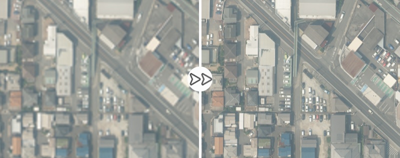
An example of super-resolution
⚠️
cf. @solafune(https://solafune.com)
Use for any purpose other than participation in the competition or commercial use is prohibited.
If you would like to use them for any of the above purposes, please contact us.
Algorithms
The algorithm we use is ESPCN. To introduce this algorithm, we will first explain the use of deep learning in a single image super-resolution.
SRCNN
As the name suggests, this algorithm applies CNN to the super-resolution task. It resizes a low-resolution image to the same size as a high-resolution image and passes it through 3 to 5 layers of CNN to increase the resolution.
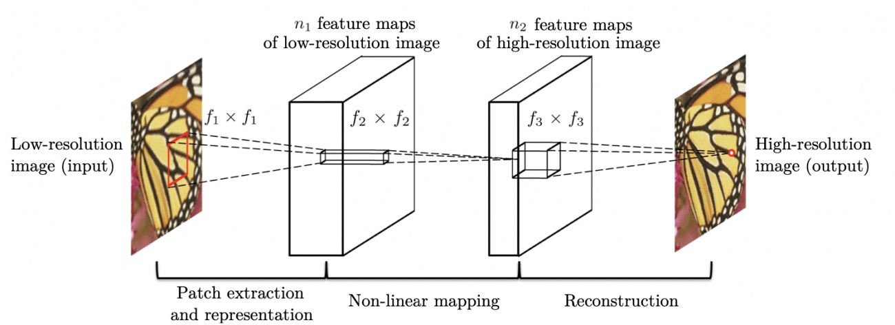
source:https://arxiv.org/pdf/1501.00092.pdf
FSRCNN
This algorithm was invented by the developers of SRCNN to spped it up. In SRCNN, the need to resize low-resolution images beforehand has been an issue for time improvement. Therefore, FSRCNN increases the resolution by performing deconvolution on the last layer of the neural network to solve this issue.
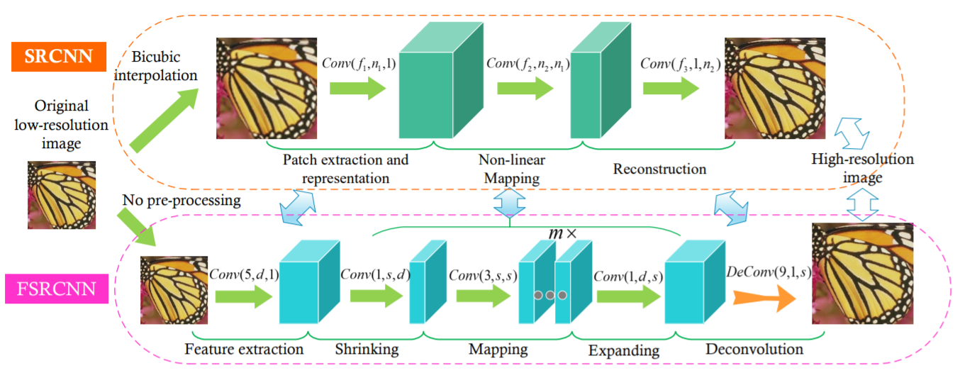
source:https://arxiv.org/pdf/1608.00367.pdf
ESPCN
FSRCNN used deconvolution to increase the resolution, but the generated image may show speckled patterns. To improve the images, ESPCN uses an algorithm called Sub-Pixel Convolution (Pixel Shuffle) instead of deconvolution.
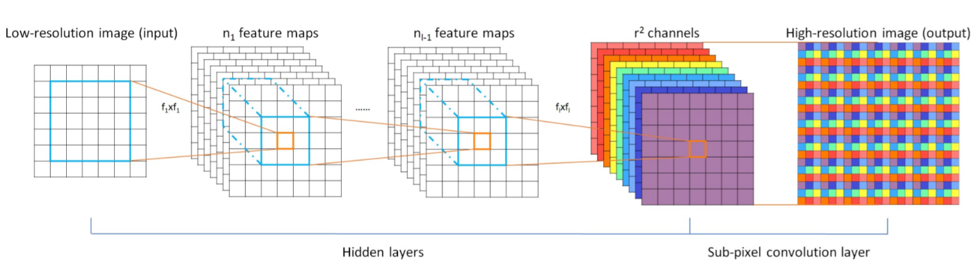
source:https://arxiv.org/pdf/1609.05158.pdf
This algorithm has had a significant impact on the development of later algorithms, such as SRResnet.
Baseline
License
The program we used follows Apache License 2.0.
The ESPCN referred to is also available under the Apache License 2.0.
Copyright 2021 @Solafune

Licensed under the Apache License, Version 2.0 (the "License");
you may not use this file except in compliance with the License.
You may obtain a copy of the License at

http://www.apache.org/licenses/LICENSE-2.0

Unless required by applicable law or agreed to in writing, software
distributed under the License is distributed on an "AS IS" BASIS,
WITHOUT WARRANTIES OR CONDITIONS OF ANY KIND, either express or implied.
See the License for the specific language governing permissions and
limitations under the License.
Directory structure
┣━ train
┃  ┗━ train_*.tif
┣━ evaluation
┃  ┗━ evaluation_*.tif
┣━ output
┃  ┗━ test_*.tif
┗━ ESPCN_sample.py
Development Configuration
- Computer specs
- CPU: Intel Core i5-6500
- RAM: 8GB
- GPU: Geforce GTX 1070
- Development environment
- We used Docker to develop the environment. Dockerfile is as follows:
FROM tensorflow/tensorflow:latest-gpu
RUN pip install Pillow
- We also checked that this also works on Google Colaboratory. In this case, you need to add/change the code for the file path and Google Drive mount.
Code Description
Libraries
You import the required libraries.
import os

os.environ["TF_FORCE_GPU_ALLOW_GROWTH"]= "true"

import tensorflow as tf
import tensorflow.keras.layers as kl
from tensorflow.python.keras import backend as K
import numpy as np
from PIL import Image
Model
This is the ESPCN model to be used in the baseline. ESPCN performs upsampling using Sub-Pixel Convolution, which is not included in Tensorflow by default, so you need to implement it by yourself.
# ESPCN
class ESPCN(tf.keras.Model):
    def __init__(self, input_shapes):
        super().__init__()

        self.input_shape_lm = ( None, input_shapes[0], input_shapes[1], 3)
        self.upsampling_scale = 4

        self.conv_0 = kl.Conv2D(64, 5, padding="same", activation="relu", input_shape=self.input_shape_lm)
        self.conv_1 = kl.Conv2D(32, 3, padding="same", activation="relu")
        self.pixel_shuffle = Pixel_shuffler(self.upsampling_scale, input_shapes)

    def call(self, x):
        conv2d_0 = self.conv_0(x)
        conv2d_1 = self.conv_1(conv2d_0)
        model = self.pixel_shuffle(conv2d_1)
        return model


# Pixel Shuffle
class Pixel_shuffler(tf.keras.Model):
    def __init__(self, upscale, input_shape):
        super().__init__()

				self.upscale = upscale
        self.conv = kl.Conv2D(self.upscale**2 * 3, kernel_size=3, padding="same")
        self.act = kl.Activation(tf.nn.relu)

    # forward proc
    def call(self, x):

        d1 = self.conv(x)
        d2 = self.act(tf.nn.depth_to_space(d1, self.upscale))

        return d2
Training
We train the image using Adam for the Optimizer and MSE for the loss function.
# Training
class trainer(object):
    def __init__(self, lr_shape, trained_model=""):
        self.model = ESPCN  ( lr_shape)
        self.model.compile(optimizer=tf.keras.optimizers.Adam(),
                  loss=tf.keras.losses.MeanSquaredError(),
                  metrics=[self.ssim])

        if trained_model != "":
          self.model.load_weights(trained_model)

    def train(self, lr_imgs, hr_imgs, out_path, batch_size, epochs):

        cp_callback = tf.keras.callbacks.ModelCheckpoint(out_path,
                                                 save_weights_only=True,
                                                 verbose=10)
        # Training
        his = self.model.fit(lr_imgs, hr_imgs, batch_size=batch_size, epochs=epochs, callbacks=[cp_callback])

        print("___Training finished\n\n")

        # Saving parameter
        print("___Saving parameter...")
        self.model.save_weights(out_path)
        print("___Completed successfully\n\n")

        return his, self.model

    # SSIM
    def ssim(self, h3, hr_imgs):
        return tf.image.ssim( h3, hr_imgs, max_val=1.0)
Data Loading
The data is normalized for the learning process. To increase the number of data, we also generate images that are flipped and mirrored and use them as teacher data.
# Dataset creation
def create_dataset():

    print("\n___Creating a dataset...")
    prc = ['/', '-', '\\', '|']
    cnt = 0
    training_data =[]

    for i in range(60):
        d = "./train/"

        # High-resolution image
        img = Image.open(d+"train_{}_high.tif".format(i))
        flip_img = np.array(ImageOps.flip(img))
        mirror_img = np.array(ImageOps.mirror(img))
        img = np.array(img)
        img = (tf.convert_to_tensor(img, np.float32)) / 255.0
        flip_img = (tf.convert_to_tensor(flip_img, np.float32)) / 255.0
        mirror_img = (tf.convert_to_tensor( mirror_img, np.float32)) / 255.0

        # Low-resolution image
        low_img = Image.open(d+"train_{}_low.tif".format(i))
        low_flip_img = np.array(ImageOps.flip(low_img))
        low_mirror_img = np.array(ImageOps.mirror(low_img))
        low_img = np.array( low_img)
        low_img = (tf.convert_to_tensor( low_img, np.float32)) / 255.0
        low_flip_img = (tf.convert_to_tensor(   low_flip_img, np.float32)) / 255.0
        low_mirror_img = (tf.convert_to_tensor( low_mirror_img, np.float32)) / 255.0

        training_data.append([img,low_img])
        training_data.append([flip_img,low_flip_img])
        training_data.append([mirror_img,low_mirror_img])

        cnt += 1

        print("\rLoading LR-images and HR-images...{}    ({} / {})".format(prc[cnt%4], cnt, 60), end='')

    print("\rLoading LR-images and HR-images...Done    ({} / {})".format(cnt, 60), end='')
    print("\n___Completed successfully\n")

    random.shuffle(training_data)
    lr_imgs = []
    hr_imgs = []

    for hr, lr in training_data:
      lr_imgs.append(lr)
      hr_imgs.append(hr)

    return np.array(lr_imgs), np.array(hr_imgs)
Implementation
We will implement the training using the functions and classes defined above. This time, batch_size is set to 15, and epochs are set to 1400. You may need to change these depending on your environment.
# Loading dataset
lr_imgs, hr_imgs = create_dataset()

print("___Start training...")
Trainer = trainer(lr_imgs[0].shape)
his, model = Trainer.train(lr_imgs, hr_imgs, out_path="espcn_model_weight" , batch_size=15, epochs=1400)
Inference
The images used for inference are normalized in the same way as when loading the data. It means that the images resulting from the inference are also normalized, so we adjust them to be in the same format as the original images.
for i in range(40):
    d = "./evaluation/"

    # Low-resolution image
    img = np.array(Image.open(d+"test_{}_low.tif".format(i)))
    img = (tf.convert_to_tensor( img, np.float32)) / 255.0
    img = img[np.newaxis, :, :, :]

    re = model.predict(img)
    re = np.reshape(re, (1200, 1500, 3))
    re = re * 255.0
    re = np.clip(re, 0.0, 255.0)
    sr_img = Image.fromarray(np.uint8(re))

    sr_img.save("./output/test_{}_answer.tif".format(i))
    print("Saved ./output/test_{}_answer.tif".format(i))
Summary
In the baseline, we used ESPCN to test the super-resolution technique. It took several hours to a day to learn, depending on the environment.
Due to the large size of the high-resolution images used in the competition, many algorithms have not been tested which require large memory to build the neural network.
Also, the score may be improved by changing the loss function, optimization method, learning coefficient, etc.
We hope this baseline helps participants more from various perspectives. Thanks!
Join now!→ "Super-resolution of City Images #MScup"
Discussion