🚀

CausalImpact の概要と Python による実装、その評価

2024/06/30に公開

Python

統計

効果検証

tech

1. 背景

ある商品の KPI (Key Performance Index) を達成するために行ったビジネスアクションを介入（施策）という。介入の効果を正しく評価するためには、施策を行った母集団のセレクションバイアスに気を付けて、RCT (Randomized Controlled Trial) を満たした手法で検証を行う必要がある。しかし、RCT を満たした手法で検証を行うのは、要求されるデータ量の大きさなどの観点から現実的には困難である。限られたデータの中で有意な検証を行う方法はいくつか存在する。そこで本記事では、その 1 つの手法である CausalImpact の概要と Python による実装について記す。実装は https://github.com/mae-commits/causal_impact_try を参照。

2. 概要

CausalImpact は DID という検証手法の考え方を応用しており、この手法と比較されることが多い。そこで、本節ではまず DID の概要を説明し、DID と比較した際の CausalImpact の利点について述べる。

2.1. 差分の差分法 (Difference in difference, DID)

DID は介入が行われた (処置群)・行われていない (コントロール群) 2 つの群に対して介入前後のデータ同士の差分を取る (Figure 1)。

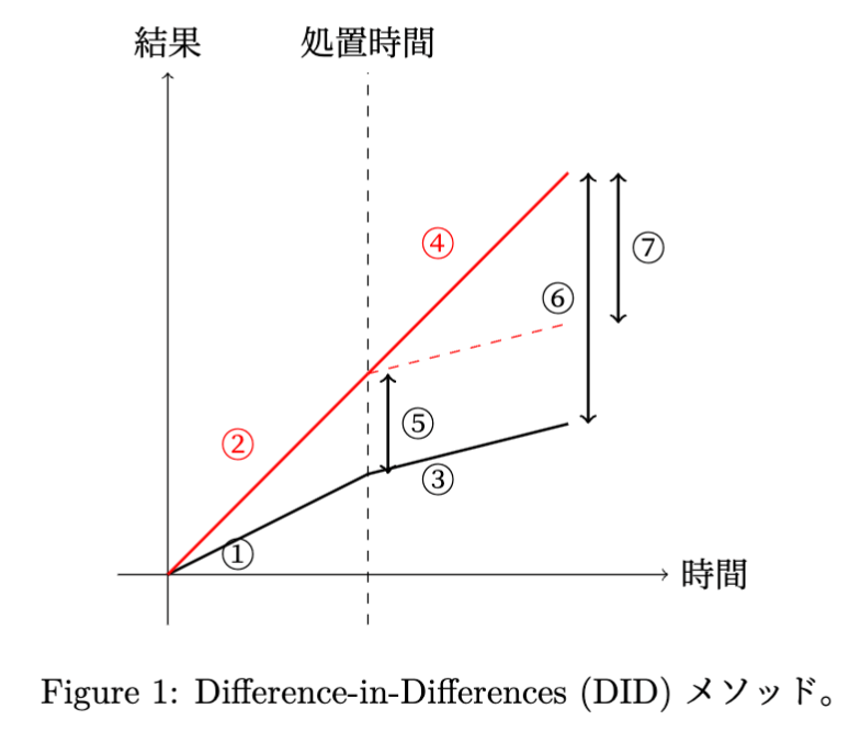
① コントロール群（事前）: コントロール群の事前期間の結果。
② 処置群（事前）: 処置群の事前期間の結果。
③ コントロール群（事後）: コントロール群の事後期間の結果。
④ 処置群（事後）: 処置群の事後期間の結果。
⑤ $\Delta$ 事前: 事前期間の処置群とコントロール群の差。
⑥ $\Delta$ 事後: 事後期間の処置群とコントロール群の差。
⑦ DID: Difference-in-Differences、つまり事後期間と事前期間の差の差。

2.1.1. メリット

差分を取ることで、地域差というセレクションバイアスをうまく省いた検証ができる。

2.1.2. デメリット

差分を取る 2 つのサンプル同士において、介入が行われていない場合にどちらも同様の傾向で変化することが予想される「平行トレンド仮定」が前提となる。また、複数地域のデータがない場合には検証できない。

2.2. CausalImpact

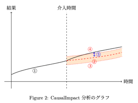
CausalImpact は、共変量 $X$ と目的変数 $Y$ のモデルを他の商品での推移を学習して、該当商品に対して介入がなかった場合の予測を行う (Figure 2)。

① 実データ: 介入前後の実際の観測データ。
② 予測データ: 介入がなかった場合の予測データ（介入後の予測）。
③ 予測区間下限: 予測データの下限範囲。
④ 予測区間上限: 予測データの上限範囲。
⑤ 影響: 介入後の実データと予測データの差。

2.2.1. メリット

複数地域のデータが必要ない。

2.2.2. デメリット

ある介入の効果の程度を適切に評価するため、共変量が介入の影響を受けないように選定する必要がある。また、複数の介入が同時に行われた場合、それぞれの効果を識別することが難しい場合がある。さらに、モデルの前提条件に強く依存しており、不適切な前提条件が結果に大きく影響する可能性がある。

3. 実装

CausalImpact の Python での実装を記す。Python のパッケージでは、tfcausalImpact が有用（2024 年6月現在）。本記事では、カリフォルニア州のタバコ「カリフォルニア禁煙キャンペーン」の因果効果を分析する。なお、データセットの定義は https://cran.r-project.org/web/packages/Ecdat/Ecdat.pdf に記載されている。

3.1. 下準備

必要なパッケージのインストール・インポート

from google.colab import drive
drive.mount('/content/drive')

import os
os.chdir('/content/drive/MyDrive/Colab_Notebooks')

# install necessary packages
!pip install tfcausalimpact pandas==1.5.0 numpy

import pandas as pd
from causalimpact import CausalImpact
import matplotlib.pyplot as plt

3.2. データ整形

データの確認

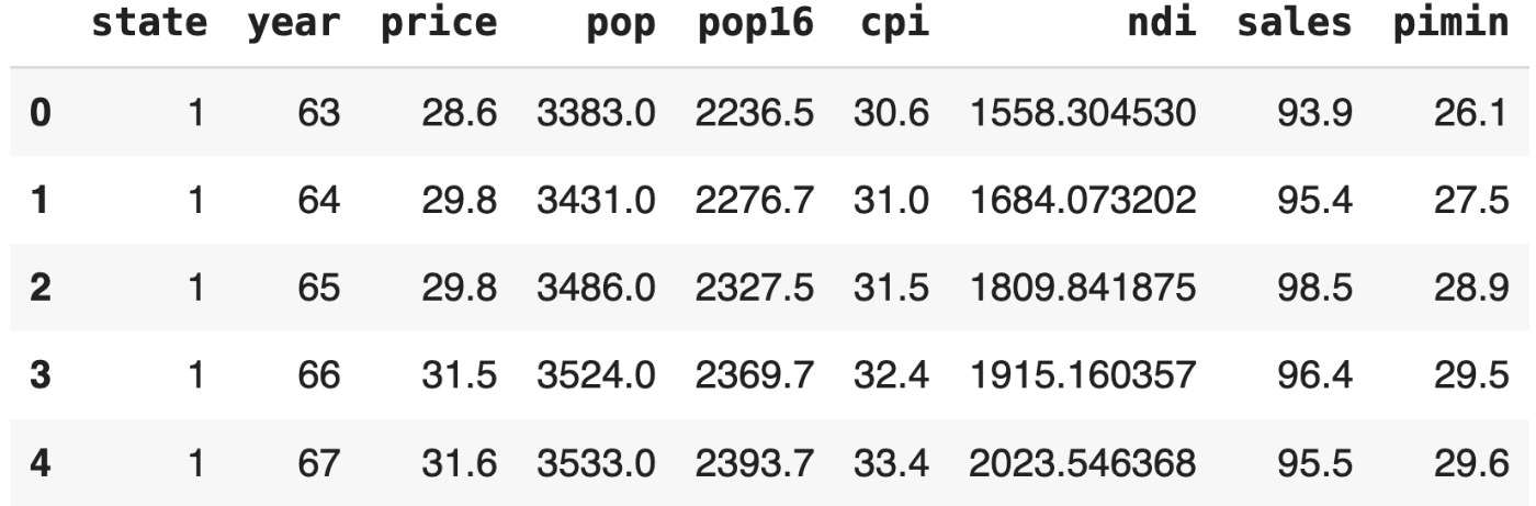
# Read dataset as pandas dataset
cigar = pd.read_csv('/content/drive/MyDrive/Colab_Notebooks/data/cigar.txt',
                   header=None,
                   sep='\s',
                   names=['state', 'year', 'price', 'pop', 'pop16', 'cpi', 'ndi', 'sales','pimin']
                   ).dropna()
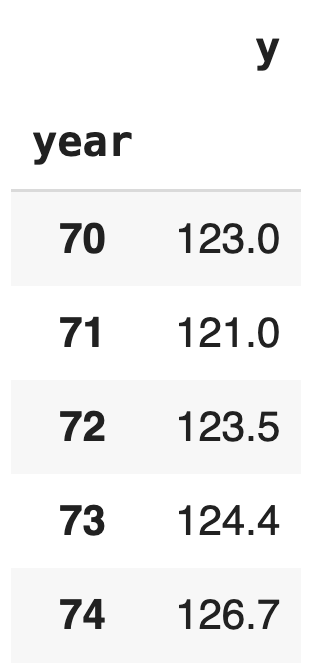
cigar.head()

列の定義 (参照：https://cran.r-project.org/web/packages/Ecdat/Ecdat.pdf )

列名	説明
state	州の略称
year	年
price	タバコ1パックあたりの価格
pop	人口
pop16	16歳以上の人口
cpi	消費者物価指数（1983年=100）
ndi	一人当たりの可処分所得
sales	一人当たりのタバコ販売量（パック）
pimin	隣接する州のタバコ1パックあたりの最低価格

禁煙キャンペーンを実施した州

州名
アリゾナ
オレゴン
フロリダ
マサチューセッツ

1988年以降にタバコ税が50セント以上増加した州

州名
アラスカ
ハワイ
メリーランド
ミシガン
ニュージャージー
ニューヨーク
ワシントン

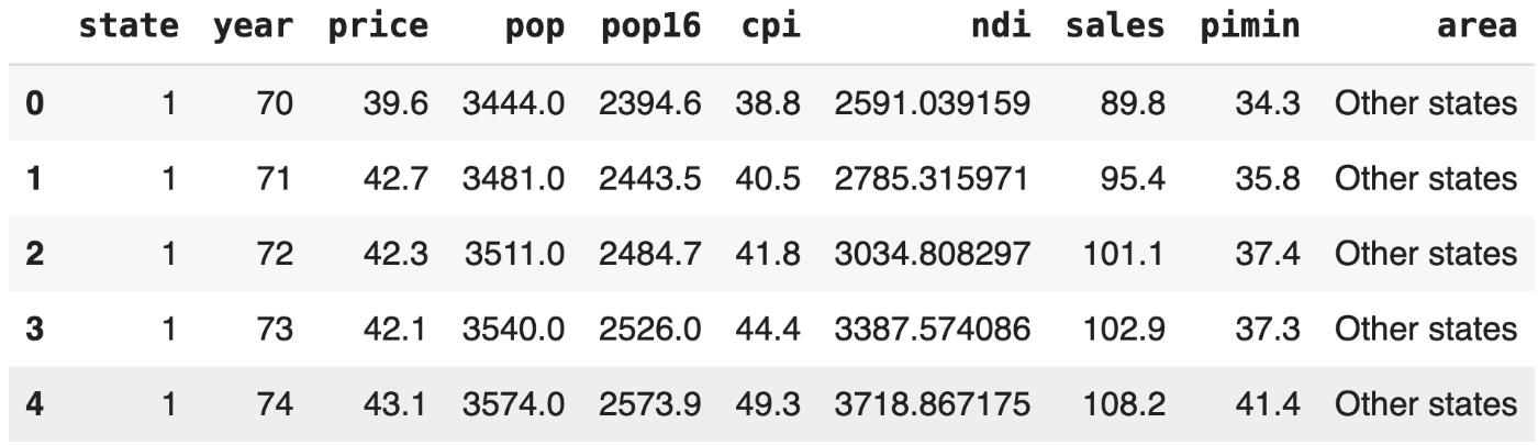
本検証では、1988 年以降にタバコ税を 50 セント以上増税した州のデータは目的とする介入以外の効果として影響を及ぼす可能性があるため、除外する。

# Skip states because they had conducted tax increase campaign after 1988,
# which may cause the other impacts except for those of our comsumption.
skip_state = [3,9,10,22,21,23,31,33,48]
cigar = cigar[(~cigar['state'].isin(skip_state)) & (cigar['year'] >= 70)].reset_index(drop=True)
cigar['area'] = cigar['state'].apply(lambda x: 'CA' if x == 5 else 'Other states')
cigar.head()cigar.head()

# Divide datasets of California for 'year' and 'sales'.
y = cigar[cigar.state == 5][['year', 'sales']].set_index('year')
y.columns = ['y']
y.head()

# Create a pivot table other than those in California
X = pd.pivot_table(cigar[cigar.state != 5][['year', 'state', 'sales']], values='sales', index='year', columns='state').add_prefix('X_')

期間の指定

禁煙キャンペーンを行ったのは、88 年であるので、介入 = 88 。このことから処理前と処理後の期間を指定する。

# Set periods
# Campaign performed in 1988. That's why 'pre_period' ends 87
pre_period = [0, 17]
post_period = [18, 22]

df_final = pd.concat([y, X], axis=1)
df_final.head()

介入の影響が共変量に対しても及んでいないかの確認

共変量として用いたデータ中で介入の影響を受けているものがないかを確認する。

# Plotting
plt.figure(figsize=(10, 6))

# Plot each column except 'y'
for column in columns:
    plt.plot(df_final.index, df_final[column], label=column)

# Add a vertical dashed line at year 88
plt.axvline(x=88, color='gray', linestyle='--', label='intervention')

# Set labels
plt.xlabel('year')
plt.ylabel('sales')
plt.legend(loc='upper center', bbox_to_anchor=(0.5, -0.15), ncol=5)

# Display the plot
plt.show()

グラフより X_30 カラムは明らかに介入前後で売上が下降していると考えられるので、カラムから外す。

df_final = df_final.drop(columns=['X_30'])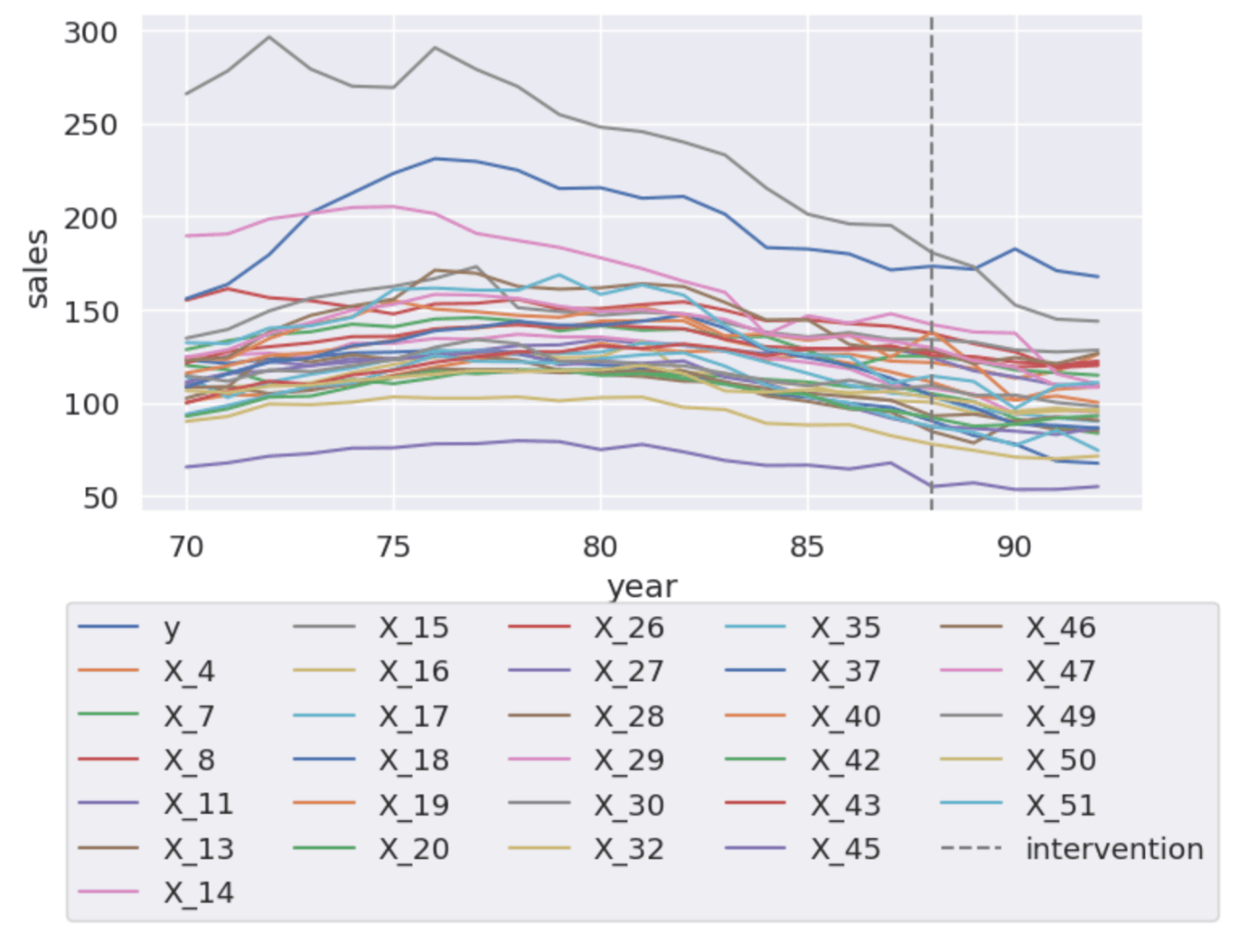

3.3. CausalImpact の実行

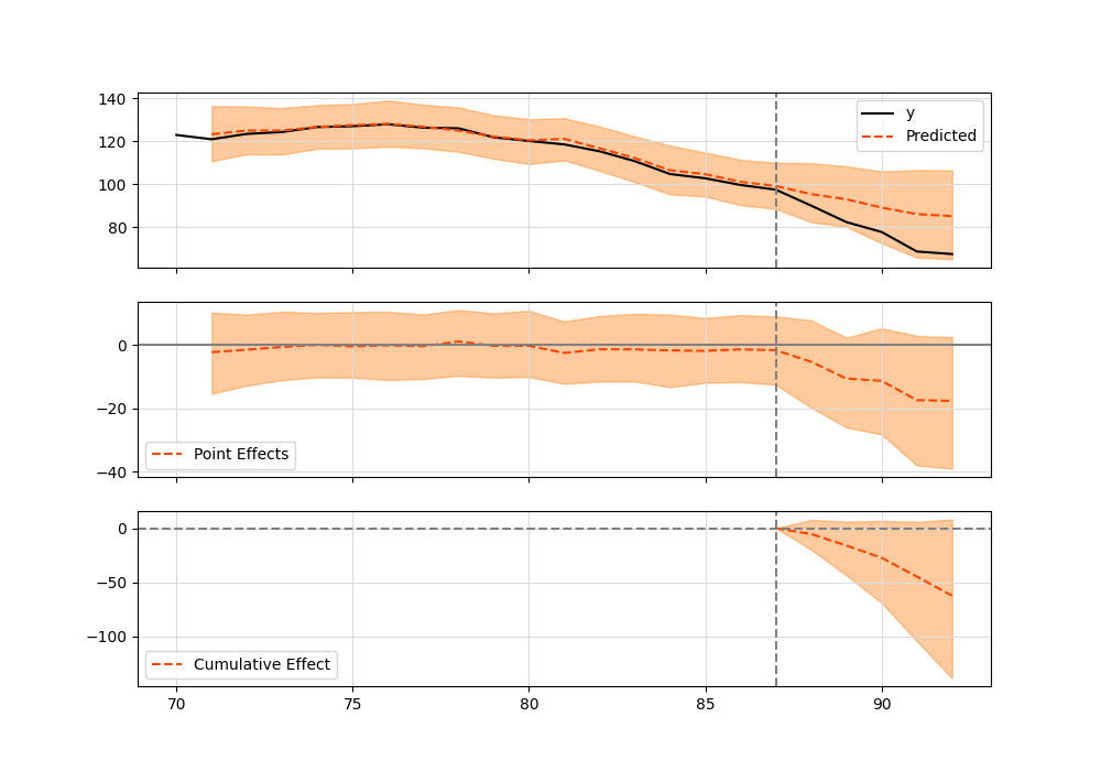
描画

# model is Hamiltonian Monte Carlo algorithm
ci = CausalImpact(df_final, pre_period, post_period, model_args={'fit_method': 'hmc'})
ci.plot()

summary 表示

print(ci.summary())

causalImpact ライブラリでは、summary() で推定値や絶対誤差、相対誤差の計算が可能。Posterior prob. of a causal effect: が介入による効果の確率を表している。
　なお、比較のために前節で確認した介入の影響を受けている可能性の高いカラムを落とした場合と落とさなかった場合を示している。

X_30 カラムを落とさなかった場合

Posterior Inference {Causal Impact}
                          Average            Cumulative
Actual                    77.3               386.5
Prediction (s.d.)         90.02 (6.72)       450.12 (33.6)
95% CI                    [74.26, 100.6]     [371.29, 502.99]

Absolute effect (s.d.)    -12.72 (6.72)      -63.62 (33.6)
95% CI                    [-23.3, 3.04]      [-116.49, 15.21]

Relative effect (s.d.)    -14.13% (7.46%)    -14.13% (7.46%)
95% CI                    [-25.88%, 3.38%]   [-25.88%, 3.38%]

Posterior tail-area probability p: 0.04
Posterior prob. of a causal effect: 96.2%

X_30 カラムを落とした場合

Posterior Inference {Causal Impact}
                          Average            Cumulative
Actual                    77.3               386.5
Prediction (s.d.)         89.79 (7.31)       448.97 (36.55)
95% CI                    [76.3, 104.96]     [381.52, 524.81]

Absolute effect (s.d.)    -12.49 (7.31)      -62.47 (36.55)
95% CI                    [-27.66, 1.0]      [-138.31, 4.98]

Relative effect (s.d.)    -13.91% (8.14%)    -13.91% (8.14%)
95% CI                    [-30.81%, 1.11%]   [-30.81%, 1.11%]

Posterior tail-area probability p: 0.04
Posterior prob. of a causal effect: 96.1%

3.4. 解釈

これらの結果を比較すると、X_30カラムを落とさなかった場合と落とした場合の両方で、実際の値と予測値の間に有意な差がある。

X_30 カラムを落とさなかった場合
平均絶対効果: -12.72 (標準偏差6.72)
相対効果: -14.13% (標準偏差7.46%)
累積絶対効果: -63.62
95%信頼区間: [-23.3, 3.04]
因果効果の確率: 96.2%
X_30 カラムを落とした場合
平均絶対効果: -12.49 (標準偏差7.31)
相対効果: -13.91% (標準偏差8.14%)
累積絶対効果: -62.47
95%信頼区間: [-27.66, 1.0]
因果効果の確率: 96.1%
比較の要点
効果の大きさは、どちらの場合も非常に近い（絶対効果は約-12.5、相対効果は約-14%）。
標準偏差および信頼区間も似ているが、X_30カラムを落とした場合の信頼区間はやや広い。
因果効果の確率はどちらも96%前後で、ほぼ同じ。
これらの結果から、X_30カラムを含めるかどうかは、因果効果の推定に大きな影響を与えないことが示唆される。

今回の検証では X_30 カラムの影響はほとんどなかったことがわかる。

3.5. 確認

確認のため、介入が行われた時期を 85 にずらしてみる。結果は以下。

summary() の出力

Posterior Inference {Causal Impact}
                          Average            Cumulative
Actual                    83.39              583.7
Prediction (s.d.)         93.34 (8.34)       653.41 (58.39)
95% CI                    [73.92, 106.62]    [517.47, 746.34]

Absolute effect (s.d.)    -9.96 (8.34)       -69.71 (58.39)
95% CI                    [-23.23, 9.46]     [-162.64, 66.23]

Relative effect (s.d.)    -10.67% (8.94%)    -10.67% (8.94%)
95% CI                    [-24.89%, 10.14%]  [-24.89%, 10.14%]

Posterior tail-area probability p: 0.11
Posterior prob. of a causal effect: 89.41%

summary(output="report") の出力

Analysis report {CausalImpact}


During the post-intervention period, the response variable had
an average value of approx. 83.39. In the absence of an
intervention, we would have expected an average response of 93.61.
The 95% interval of this counterfactual prediction is [79.24, 106.02].
Subtracting this prediction from the observed response yields
an estimate of the causal effect the intervention had on the
response variable. This effect is -10.22 with a 95% interval of
[-22.64, 4.14]. For a discussion of the significance of this effect,
see below.


Summing up the individual data points during the post-intervention
period (which can only sometimes be meaningfully interpreted), the
response variable had an overall value of 583.7.
Had the intervention not taken place, we would have expected
a sum of 655.24. The 95% interval of this prediction is [554.71, 742.15].


The above results are given in terms of absolute numbers. In relative
terms, the response variable showed a decrease of -10.92%. The 95%
interval of this percentage is [-24.18%, 4.42%].
This means that, although it may look as though the intervention has
exerted a negative effect on the response variable when considering
the intervention period as a whole, this effect is not statistically
significant and so cannot be meaningfully interpreted.


The apparent effect could be the result of random fluctuations that
are unrelated to the intervention. This is often the case when the
intervention period is very long and includes much of the time when
the effect has already worn off. It can also be the case when the
intervention period is too short to distinguish the signal from the
noise. Finally, failing to find a significant effect can happen when
there are not enough control variables or when these variables do not
correlate well with the response variable during the learning period.


The probability of obtaining this effect by chance is p = 7.59%.
This means the effect may be spurious and would generally not be
considered statistically significant.

出力結果のグラフ

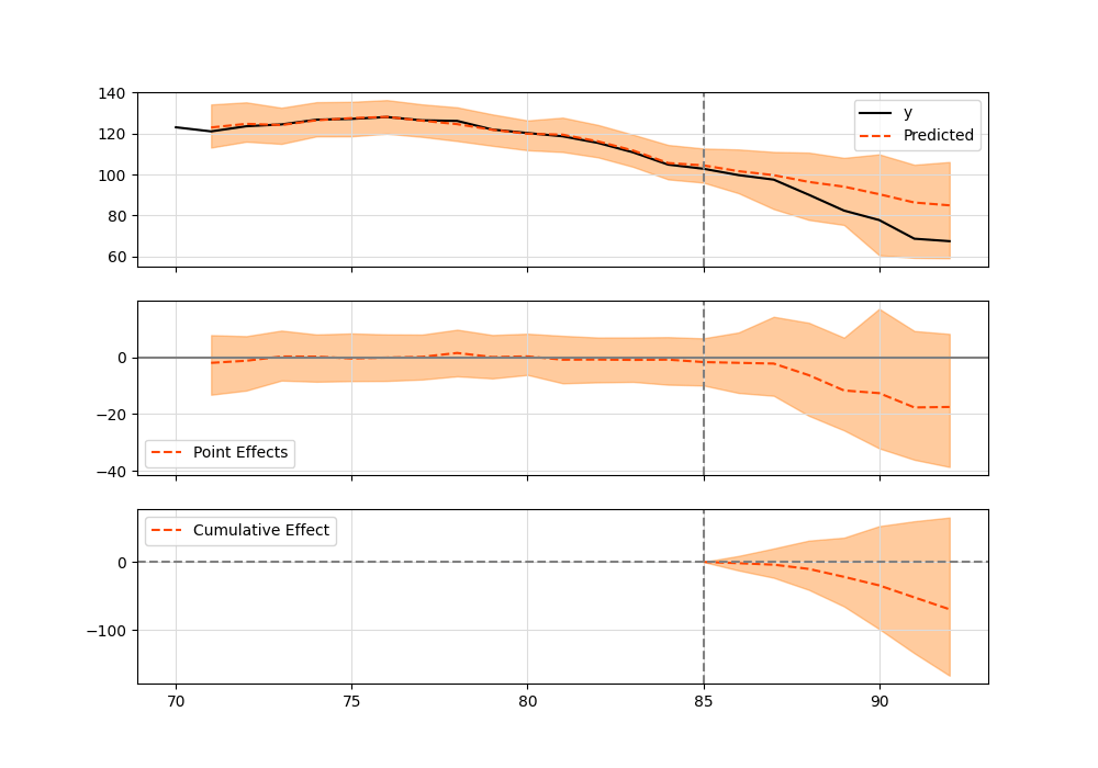
summary(output="report") の結果から、介入効果が起こる偶然の確率は 7.59 % であり、有意水準 95 % の検定では有意なものとは言えない。また、介入時期をずらす前の 95 % 信頼区間に対して値の幅が正の方向に大きくなっており、売上が減少するという結果からずれている。

4. 注意点

tfcausalImpact では、index をカラムから指定すると、datetime 型ではないと認識されずに Input data is empty. とエラー出力する可能性がある。そのため、今回は year カラムを最後に落とし、デフォルトの index として判定させるようにした。

5. まとめ

本記事では、CausalImpact の意義と Python による具体的な実装を行った。共変量の選定の仕方に関してはより詳細な選定が必要だと考えられる。以下に本記事の概要をまとめる。

介入の定義
介入前期間（Pre-period）: 介入が行われる前の期間。通常、長期間のデータが必要。
介入後期間（Post-period）: 介入が行われた後の期間。
予測と実際の値の比較
実際の値（Actual）: 介入後に観測された実際のデータ。
予測値（Prediction）: 介入がなかった場合に予測されるデータ。これは介入前のデータに基づいてモデルが予測する。
効果の測定
絶対効果（Absolute effect）: 実際の値と予測値の差。これは介入の結果としての変化を直接的に示す。
相対効果（Relative effect）: 絶対効果を予測値で割った値。これは介入の結果としての変化をパーセンテージで示す。
統計的有意性
95%信頼区間（95% CI）: 効果の推定範囲。信頼区間がゼロを含まない場合、効果が統計的に有意であると解釈される。
事後確率（Posterior probability）: 効果が存在する確率。高い事後確率は介入の効果が実際に存在する可能性を示す。
報告の要素
実際の平均値と累積値（Actual Average and Cumulative）: 介入後に観測された実際のデータの平均と累積値。
予測値の平均と累積値（Prediction Average and Cumulative）: 介入がなかった場合に予測されるデータの平均と累積値。
効果の平均と累積値（Effect Average and Cumulative）: 実際の値と予測値の差の平均と累積値。
結果の解釈
因果効果の解釈: 実際の値が予測値よりもどの程度変化したかを理解する。効果の大きさと方向（増加か減少か）を示す。
統計的有意性の確認: 信頼区間と事後確率を確認し、効果が統計的に有意かどうかを判断する。

6. 参考文献

tfcausalimpact の github repository

CausalImpact
CausalImpact をまとめた自分のブログ

第4章差分の差分法 (DID) とCausalImpact
CausalImpact で参考になる文献（R で実装している文献だが、最初の考え方の部分は参考になる）

CausalImpact
本実装の github repository
https://github.com/mae-commits/causal_impact_try