tidymodelsを使った線形回帰
この記事について
tidymodelsを使った線形回帰の練習です。
コードを実行している手もとの環境でoptions(warnPartialMatchArgs = TRUE)としているので、ところどころ「部分的な引数のマッチング」というwarningが出ていますが、気にしないでください。
suppressPackageStartupMessages({
  require(tidymodels)
  require(DALEXtra)
})
tidymodels_prefer()
#> Warning in conflicted::conflict_prefer("update", winner =
#> "recipes", loser = "Matrix", : 'loser' の 'losers'
#> への部分的な引数のマッチング
使用するデータ
openintroのmariokartというデータセットを使います。
OpenIntroというのは、高校から学部1~2年レベルくらいの統計の教科書を書いているプロジェクトです。mariokartは、その教科書のために用意されたサンプルデータのひとつ。なお、この教科書は『データ分析のための統計学入門』として邦訳されています。
data("mariokart", package = "openintro")
mariokart <- mariokart |>
  dplyr::select(
    total_pr, duration, n_bids, cond, ship_sp, stock_photo,
    wheels, start_pr, seller_rate
  )

skimr::skim_tee(mariokart)
#> ── Data Summary ────────────────────────
#>                            Values
#> Name                       data
#> Number of rows             143
#> Number of columns          9
#> _______________________
#> Column type frequency:
#>   factor                   3
#>   numeric                  6
#> ________________________
#> Group variables            None
#>
#> ── Variable type: factor ───────────────────────────────────
#>   skim_variable n_missing complete_rate ordered n_unique
#> 1 cond                  0             1 FALSE          2
#> 2 ship_sp               0             1 FALSE          8
#> 3 stock_photo           0             1 FALSE          2
#>   top_counts
#> 1 use: 84, new: 59
#> 2 sta: 33, ups: 31, pri: 23, fir: 22
#> 3 yes: 105, no: 38
#>
#> ── Variable type: numeric ──────────────────────────────────
#>   skim_variable n_missing complete_rate     mean        sd
#> 1 total_pr              0             1    49.9     25.7
#> 2 duration              0             1     3.77     2.59
#> 3 n_bids                0             1    13.5      5.88
#> 4 wheels                0             1     1.15     0.847
#> 5 start_pr              0             1     8.78    15.1
#> 6 seller_rate           0             1 15898.   51840.
#>      p0    p25   p50    p75     p100 hist
#> 1 29.0   41.2   46.5   54.0    327.  ▇▁▁▁▁
#> 2  1      1      3      7       10   ▇▅▂▆▁
#> 3  1     10     14     17       29   ▂▅▇▃▁
#> 4  0      0      1      2        4   ▆▇▇▁▁
#> 5  0.01   0.99   1     10       70.0 ▇▁▁▁▁
#> 6  0    109    820   4858   270144   ▇▁▁▁▁
mariokartは、eBayにおける2009年10月中のアメリカからの出品について、「マリオカートWii」の出品を収集したもの。ここでは次の列を使って、total_prを目的変数とした回帰をおこないます。
- total_pr: 落札価格(送料含む)
- duration: オークションの期間(単位:日)
- n_bids: 入札回数
- cond: 出品が中古かどうか
- ship_sp: 配送オプション
- stock_photo: 商品の写真が「ストックフォト」かどうか
- wheels: 出品に含まれる「ステアリングホイール(ハンドル型のコントローラ)」の数
- start_pr: オークションの開始価格
- seller_rate: 出品者のユーザー評価
元のデータセットは143行12列で、いずれの列にも欠損値はありませんが、total_prが外れ値になっているケースが2件あることがわかっています。
set.seed(1309)
mariokart <- mariokart |>
  initial_split(strata = total_pr, prop = 0.8)

training(mariokart) |>
  DataExplorer::plot_qq()
#> Warning in facet_wrap(facet = ~variable, nrow = 3L, ncol =
#> 3L, scales = "free_y"): 'facet' の 'facets'
#> への部分的な引数のマッチング
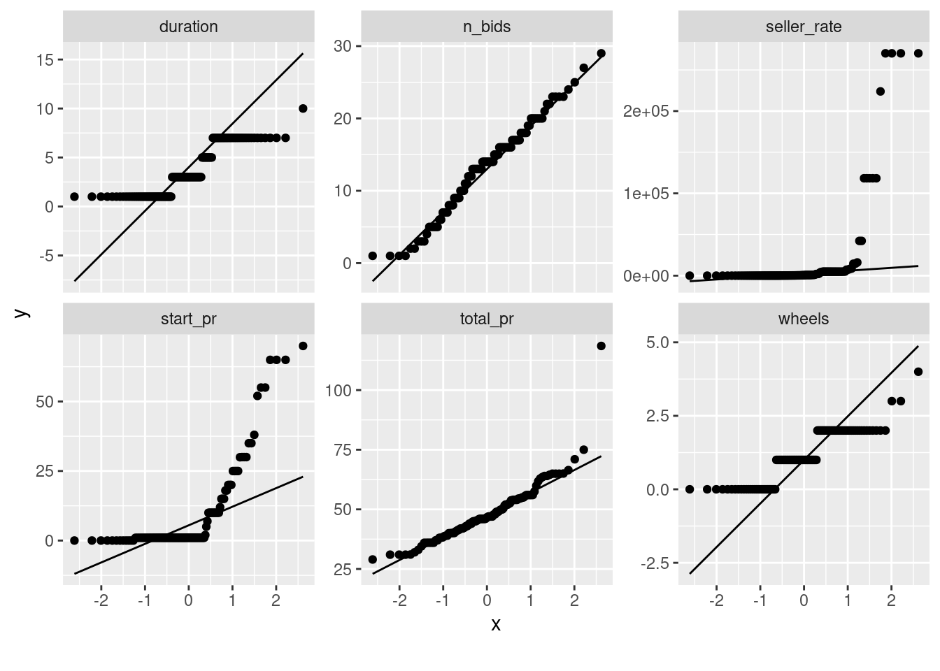
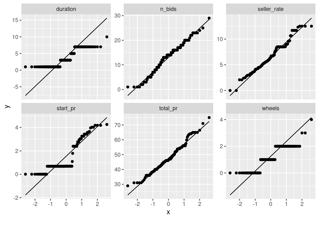
それら2件の出品は「マリオカートWii」以外のゲームソフトなどとあわせて出品されたもので、落札価格が$100を超えています。これらを除外しつつ、特徴量を適当に変換すればうまく回帰できそうです。
training(mariokart) |>
  dplyr::filter(total_pr < 100) |>
  dplyr::mutate(
    start_pr = log1p(start_pr),
    seller_rate = log1p(seller_rate)
  ) |>
  DataExplorer::plot_qq()
#> Warning in facet_wrap(facet = ~variable, nrow = 3L, ncol =
#> 3L, scales = "free_y"): 'facet' の 'facets'
#> への部分的な引数のマッチング
ship_spは水準がやや多いですが、実際にはstandardとupsGroundの割合が多く、その他のオプションはそれほど使われていないようです。
training(mariokart) |>
  dplyr::filter(total_pr < 100) |>
  DataExplorer::plot_bar()
#> Warning in facet_wrap(facet = ~variable, nrow = 3L, ncol =
#> 3L, scales = "free"): 'facet' の 'facets'
#> への部分的な引数のマッチング
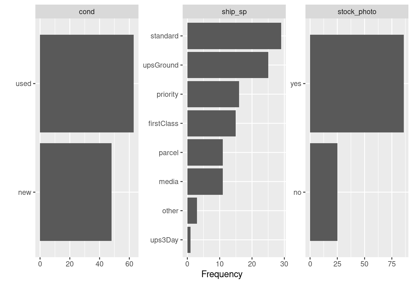
standardはeBayにおける「標準配送」で、upsGroundとups3DayはUPSを利用した配送、その他はUSPSを利用した配送だと思われます。priorityはPriority Mail(速達みたいなもの)、firstClassがFirst-Class Mail(定形郵便みたいなもの)、parcelは小包、mediaはMedia Mail(レターパックみたいなもの。本などを送るのに使う)でしょう。
前処理
とりあえず次のような前処理をおこなうことにします。
rec <- recipe(total_pr ~ ., data = training(mariokart)) |>
  step_filter(total_pr < 100, skip = TRUE) |>
  step_log(seller_rate, offset = 1) |>
  step_log(start_pr, offset = 1) |>
  step_nzv(all_predictors()) |>
  step_scale(all_numeric_predictors(), factor = 2) |>
  step_other(ship_sp, threshold = .15) |>
  step_dummy(all_nominal_predictors()) |>
  step_center(all_numeric_predictors())
recipes::step_scale(factor = 2)とすると、2標準偏差で割ってスケーリングすることができます。ダミー変数も同様のやり方でスケーリングしてよいのですが、今回のデータのように0/1が等確率でない場合、1単位の変化では同じ水準に戻らないため、スケーリングしない場合に比べて係数が若干割り引かれてしまいます。ここでは、連続変数についてのみスケーリングすることにします。
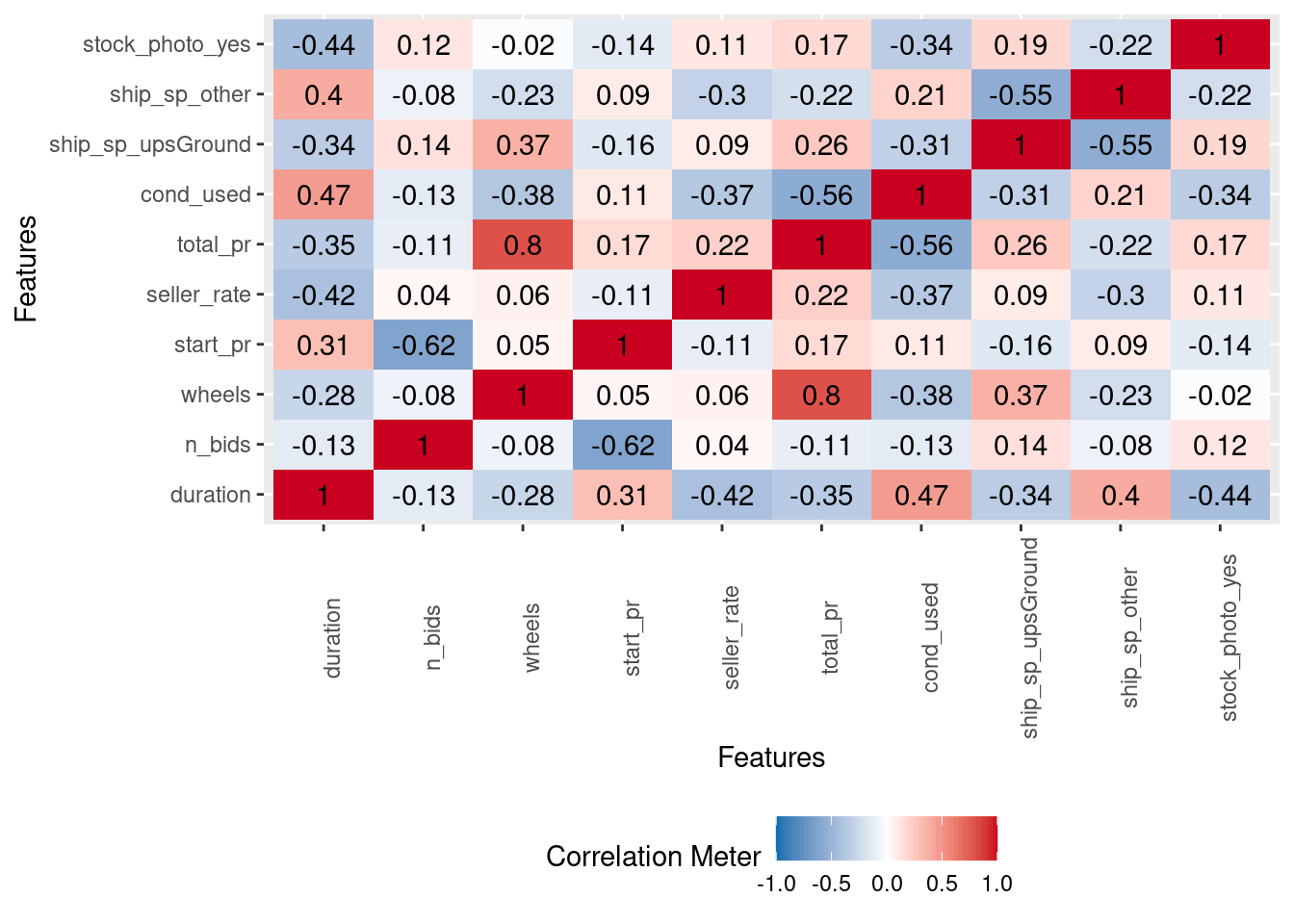
この前処理をおこなった場合に得られる特徴量間の相関は、次のようになります。
rec |>
  prep() |>
  bake(new_data = NULL) |>
  DataExplorer::plot_correlation()
モデリング
先ほどの前処理をしつつ、ふつうに線形回帰してみます。
spec <- linear_reg() |>
  set_engine("lm") |>
  set_mode("regression")

wf <- workflow() |>
  add_recipe(rec) |>
  add_model(spec) |>
  fit(training(mariokart))

tidy(wf)
#> # A tibble: 10 × 5
#>    term              estimate std.error statistic   p.value
#>    <chr>                <dbl>     <dbl>     <dbl>     <dbl>
#>  1 (Intercept)         47.7       0.444   107.    5.83e-106
#>  2 duration            -0.556     1.26     -0.442 6.59e-  1
#>  3 n_bids               0.677     1.16      0.581 5.62e-  1
#>  4 wheels              13.7       1.07     12.9   5.54e- 23
#>  5 start_pr             3.87      1.21      3.21  1.80e-  3
#>  6 seller_rate          1.60      1.07      1.50  1.36e-  1
#>  7 cond_used           -4.84      1.16     -4.16  6.79e-  5
#>  8 ship_sp_upsGround   -2.47      1.39     -1.77  7.94e-  2
#>  9 ship_sp_other       -0.222     1.15     -0.193 8.48e-  1
#> 10 stock_photo_yes      2.73      1.26      2.17  3.26e-  2
glance(wf)
#> # A tibble: 1 × 12
#>   r.squared adj.r.squared sigma statistic  p.value    df
#>       <dbl>         <dbl> <dbl>     <dbl>    <dbl> <dbl>
#> 1     0.777         0.757  4.68      39.1 4.69e-29     9
#> # ℹ 6 more variables: logLik <dbl>, AIC <dbl>, BIC <dbl>,
#> #   deviance <dbl>, df.residual <int>, nobs <int>
wheelsやcond_used, start_prが1%水準で有意なようです。start_prは対数変換していたので、1単位(2標準偏差、$30くらい)上がると$46くらい増えます。
多重共線性を確認します。
extract_fit_engine(wf) |>
  car::vif()
#>          duration            n_bids            wheels
#>          1.988910          1.705051          1.434335
#>          start_pr       seller_rate         cond_used
#>          1.829121          1.426426          1.688625
#> ship_sp_upsGround     ship_sp_other   stock_photo_yes
#>          1.718345          1.687931          1.404189
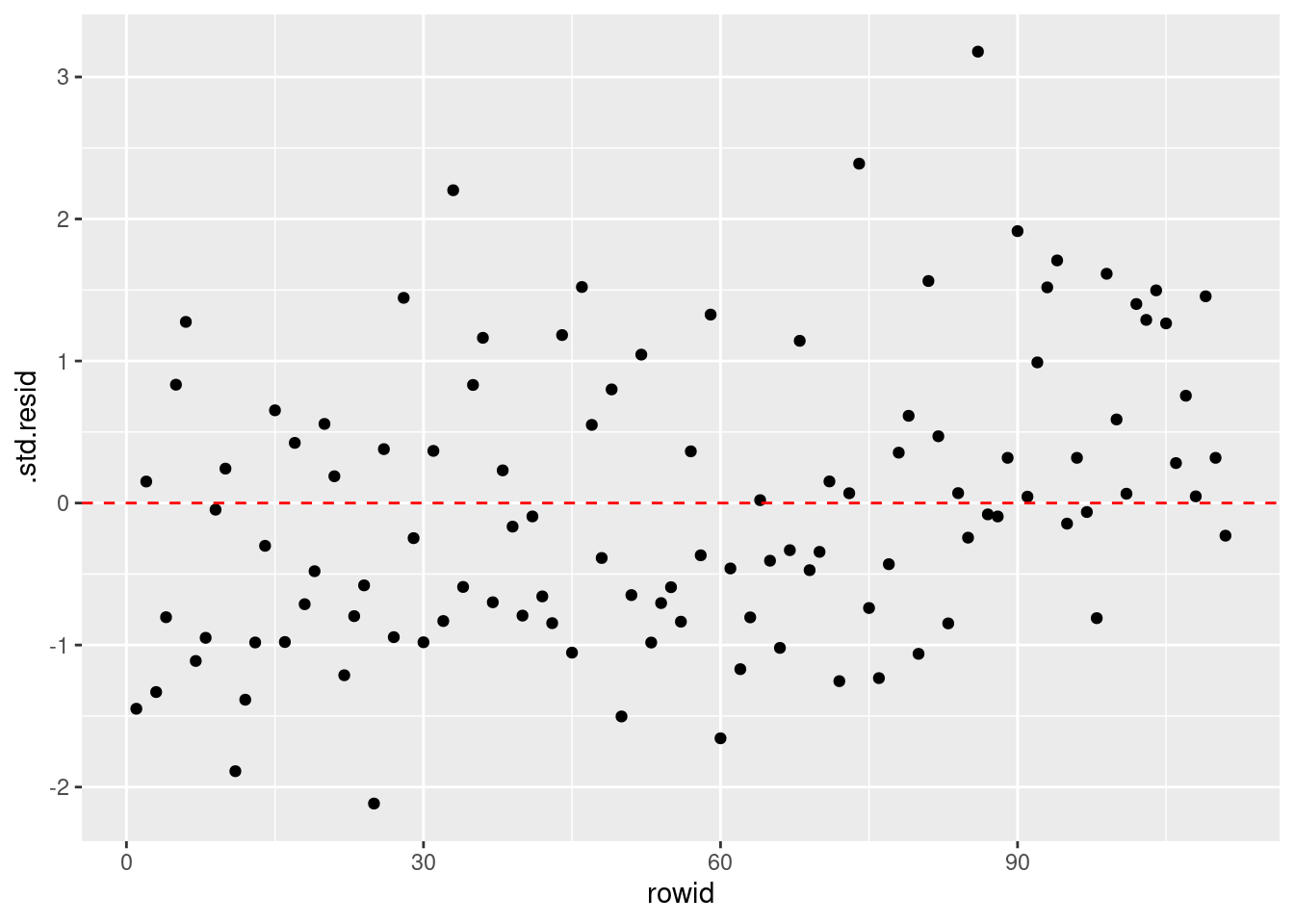
残差(ここでは標準化されている)のばらつきにおかしなパターンがないことを確認します。
extract_fit_engine(wf) |>
  augment(dplyr::filter(training(mariokart), total_pr < 100)) |>
  dplyr::mutate(rowid = row_number()) |>
  ggplot(aes(x = rowid, y = .std.resid)) +
  geom_point() +
  geom_hline(yintercept = 0, color = "red", linetype = "dashed")
前処理の調整
ship_spのどの水準までダミー変数にするかは先ほどは勘で決めただけなので、調整してみましょう。また、n_bidsはなくてもよい気がするので、投入しないrecipeもつくって比較してみます。
rec_base <- recipe(total_pr ~ ., data = training(mariokart)) |>
  step_filter(total_pr < 100, skip = TRUE) |>
  step_log(seller_rate, offset = 1) |>
  step_log(start_pr, offset = 1) |>
  step_nzv(all_predictors()) |>
  step_scale(all_numeric_predictors(), factor = 2) |>
  step_other(ship_sp, threshold = tune()) |>
  step_dummy(all_nominal_predictors()) |>
  step_center(all_numeric_predictors())

rec_no_n_bids <- rec_base |>
  step_select(!n_bids, skip = TRUE)
workflosets::workflow_mapでtune_gridします。訓練用データが112行と少ないので、ここでは、30個のブートストラップ標本を使って検証することにします。
ブートストラップ標本は訓練用データを復元抽出してつくられるので、各ブートストラップ標本をつくるステップにおいて、およそ63.2%のデータは少なくとも1回は抽出される一方、残りの36.8%程度のデータは1回も抽出されません。
rsample::bootstrapsでは、各ステップごとに、ブートストラップ標本として1回も抽出されなかったデータからなる標本(out-of-bag sample)が検証用データになります。
doFuture::registerDoFuture()
plan <- future::plan(
  "multisession",
  workers = parallelly::availableCores(omit = 4)
)

wf_sets <-
  workflow_set(
    list(
      base_rec = rec_base,
      no_n_bids = rec_no_n_bids
    ),
    list(linear_reg = spec),
    cross = TRUE
  ) |>
  workflow_map(
    "tune_grid",
    resamples = bootstraps(training(mariokart), strata = total_pr, times = 30),
    grid = withr::with_seed(1309, {
      grid_max_entropy(
        dials::threshold(range = c(0.1, 0.25)),
        size = 10
      )
    }),
    metrics = metric_set(rsq, rsq_trad)
  )

future::plan(plan)
決定係数で見るかぎりでは、n_bidsはあってもなくてもよさそうです。thresholdの値のほうは、ここで探索している範囲では、resamplesの中身次第で実際の結果が変わってしまうようで、安定しませんでした。
rank_results(wf_sets) |>
  dplyr::filter(.metric == "rsq_trad")
#> # A tibble: 20 × 9
#>    wflow_id .config .metric  mean std_err     n preprocessor
#>    <chr>    <chr>   <chr>   <dbl>   <dbl> <int> <chr>
#>  1 base_re… Prepro… rsq_tr… 0.383  0.0580    30 recipe
#>  2 base_re… Prepro… rsq_tr… 0.382  0.0582    30 recipe
#>  3 base_re… Prepro… rsq_tr… 0.380  0.0578    30 recipe
#>  4 base_re… Prepro… rsq_tr… 0.380  0.0585    30 recipe
#>  5 base_re… Prepro… rsq_tr… 0.380  0.0587    30 recipe
#>  6 base_re… Prepro… rsq_tr… 0.379  0.0591    30 recipe
#>  7 base_re… Prepro… rsq_tr… 0.379  0.0589    30 recipe
#>  8 base_re… Prepro… rsq_tr… 0.379  0.0586    30 recipe
#>  9 base_re… Prepro… rsq_tr… 0.378  0.0593    30 recipe
#> 10 base_re… Prepro… rsq_tr… 0.376  0.0568    30 recipe
#> 11 no_n_bi… Prepro… rsq_tr… 0.369  0.0608    30 recipe
#> 12 no_n_bi… Prepro… rsq_tr… 0.368  0.0609    30 recipe
#> 13 no_n_bi… Prepro… rsq_tr… 0.366  0.0603    30 recipe
#> 14 no_n_bi… Prepro… rsq_tr… 0.368  0.0617    30 recipe
#> 15 no_n_bi… Prepro… rsq_tr… 0.367  0.0618    30 recipe
#> 16 no_n_bi… Prepro… rsq_tr… 0.367  0.0615    30 recipe
#> 17 no_n_bi… Prepro… rsq_tr… 0.367  0.0613    30 recipe
#> 18 no_n_bi… Prepro… rsq_tr… 0.367  0.0617    30 recipe
#> 19 no_n_bi… Prepro… rsq_tr… 0.364  0.0593    30 recipe
#> 20 no_n_bi… Prepro… rsq_tr… 0.366  0.0614    30 recipe
#> # ℹ 2 more variables: model <chr>, rank <int>

best_params <- wf_sets |>
  extract_workflow_set_result(id = rank_results(wf_sets)[["wflow_id"]][1]) |>
  select_best(metric = "rsq_trad")

best_params
#> # A tibble: 1 × 2
#>   threshold .config
#>       <dbl> <chr>
#> 1     0.154 Preprocessor10_Model1
機械的にもっとも評価指標がよかった結果を選択するならば、上のようにしたbest_paramsをtune::finalize_workflowに渡せばよいのですが、ここではthreshold=0.10に調整することにします。
wf_fit <- wf_sets |>
  extract_workflow(id = "base_rec_linear_reg") |>
  finalize_workflow(tibble::tibble(threshold = 0.10)) |>
  last_fit(mariokart, metrics = metric_set(rmse, rsq, rsq_trad))

collect_metrics(wf_fit)
#> # A tibble: 3 × 4
#>   .metric  .estimator .estimate .config
#>   <chr>    <chr>          <dbl> <chr>
#> 1 rmse     standard    49.9     Preprocessor1_Model1
#> 2 rsq      standard     0.0422  Preprocessor1_Model1
#> 3 rsq_trad standard     0.00427 Preprocessor1_Model1
実際の評価指標がとても悪いですが、これはすでに説明したように外れ値があるためであって、必ずしもモデルが悪いせいではありません。
wf_fit |>
  extract_fit_parsnip() |>
  tidy()
#> # A tibble: 12 × 5
#>    term              estimate std.error statistic   p.value
#>    <chr>                <dbl>     <dbl>     <dbl>     <dbl>
#>  1 (Intercept)         47.7       0.446   107.    3.83e-104
#>  2 duration            -0.583     1.27     -0.461 6.46e-  1
#>  3 n_bids               0.636     1.17      0.542 5.89e-  1
#>  4 wheels              13.5       1.10     12.3   1.33e- 21
#>  5 start_pr             3.92      1.21      3.23  1.67e-  3
#>  6 seller_rate          1.66      1.07      1.55  1.26e-  1
#>  7 cond_used           -4.81      1.17     -4.11  8.04e-  5
#>  8 ship_sp_priority     0.575     1.70      0.338 7.36e-  1
#>  9 ship_sp_standard     1.14      1.57      0.724 4.71e-  1
#> 10 ship_sp_upsGround   -1.19      1.74     -0.681 4.98e-  1
#> 11 ship_sp_other        1.63      1.57      1.04  3.02e-  1
#> 12 stock_photo_yes      2.54      1.28      1.99  4.97e-  2
wf_fit |>
  extract_fit_parsnip() |>
  glance()
#> # A tibble: 1 × 12
#>   r.squared adj.r.squared sigma statistic  p.value    df
#>       <dbl>         <dbl> <dbl>     <dbl>    <dbl> <dbl>
#> 1     0.780         0.755  4.70      31.8 1.05e-27    11
#> # ℹ 6 more variables: logLik <dbl>, AIC <dbl>, BIC <dbl>,
#> #   deviance <dbl>, df.residual <int>, nobs <int>
wf_fit |>
  extract_fit_engine() |>
  car::vif()
#>          duration            n_bids            wheels
#>          1.994808          1.715311          1.504422
#>          start_pr       seller_rate         cond_used
#>          1.831740          1.437856          1.689451
#>  ship_sp_priority  ship_sp_standard ship_sp_upsGround
#>          1.792062          2.386657          2.662293
#>     ship_sp_other   stock_photo_yes
#>          2.230741          1.433650
今回のthresholdだとship_spはfirstClassが参照水準(基準カテゴリ)で、standard, upsGround, priorityとその他の水準の5つになります。どうやら、standardやpriorityよりはfirstClassのほうが(それで送れるなら)少しだけ安く、upsGroundにするとfirstClassよりもさらに安くできるようです。
効果プロット
total_prが外れ値であるケースについて、どのような予測がされているか詳しく見てみましょう。まず、先ほどのモデルでtotal_prが外れ値であるケースの落札価格を予測してみます。
preds <-
  extract_workflow(wf_fit) |>
  augment(
    openintro::mariokart |>
      dplyr::mutate(rowid = dplyr::row_number()) |>
      dplyr::filter(total_pr > 100)
  ) |>
  dplyr::select(
    rowid, title, total_pr, .pred,
    wheels, cond, ship_sp, stock_photo
  )

preds
#> # A tibble: 2 × 8
#>   rowid title            total_pr .pred wheels cond  ship_sp
#>   <int> <fct>               <dbl> <dbl>  <int> <fct> <fct>
#> 1    20 "Nintedo Wii Co…     327.  49.7      2 used  parcel
#> 2    65 "10 Nintendo Wi…     118.  36.5      0 used  parcel
#> # ℹ 1 more variable: stock_photo <fct>
rowid=20はWii本体と2つのステアリングホイールが含まれる出品で、$327という価格が付けられています。また、rowid=65は「マリオカートWii」を含む10点の中古ゲームソフトをまとめている出品で、$118の価格が付けられています。
次に、これらのケースの各特徴量の効果をデータ全体における効果の分布と一緒にプロットします。
weights <-
  wf_fit |>
  extract_workflow() |>
  tidy() |>
  dplyr::pull(estimate, name = term)

wf_fit |>
  extract_preprocessor() |>
  prep() |>
  bake(new_data = openintro::mariokart) |>
  dplyr::select(any_of(names(weights))) |>
  rlang::as_function(~ {
    ret <- t(as.matrix(.)) * weights[colnames(.)]
    rownames(ret) <- colnames(.)
    t(ret)
  })() |>
  dplyr::as_tibble() |>
  dplyr::mutate(
    id = dplyr::row_number(),
    rowid = dplyr::case_when(
      id == 20 ~ 1,
      id == 65 ~ 2,
      .default = 3
    ) |> factor(labels = c(20, 65, 0))
  ) |>
  tidyr::pivot_longer(
    cols = any_of(names(weights)),
    names_to = "term",
    values_to = "effect"
  ) |>
  dplyr::mutate(
    term = factor(term, rev(names(weights[-1])))
  ) |>
  ggplot(aes(x = term, y = effect)) +
  geom_boxplot() +
  geom_jitter(
    aes(colour = rowid),
    data = \(x) dplyr::filter(x, id %in% c(20, 65)),
    size = 2, shape = 4
  ) +
  geom_hline(aes(yintercept = 0), colour = "grey", linetype = "dashed") +
  coord_flip(ylim = c(-10, 10))

このモデルでは、wheels以外の特徴量については効果のばらつきが小さく、予測値にそれほど大きくは寄与しません。rowid=20のケースではステアリングホイールが2個含まれていたので正の効果が、rowid=65のケースではステアリングホイールは0個なので負の効果がありますが、いずれにせよ、これらのケースが高額であると予測するためには適切な特徴量が足りなかったようです。
SHAP
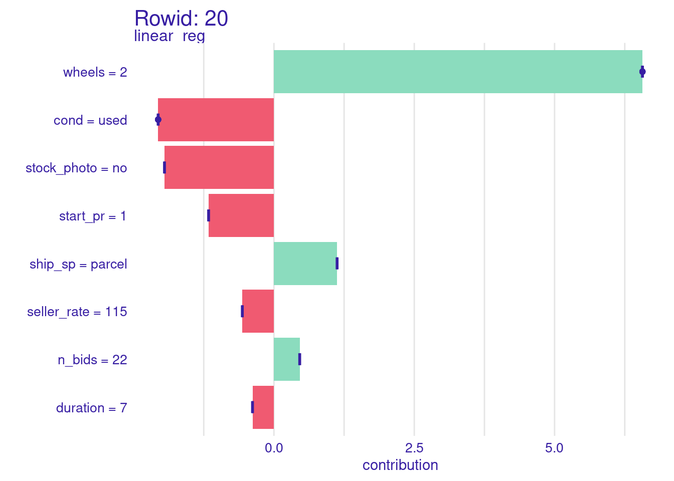
さいごに、SHAPも確認してみましょう。まず、rowid=20のもの。
explainer <-
  extract_workflow(wf_fit) |>
  explain_tidymodels(
    data = dplyr::select(training(mariokart), !total_pr),
    y = training(mariokart)[["total_pr"]],
    label = "linear_reg"
  )
#> Preparation of a new explainer is initiated
#>   -> model label       :  linear_reg
#>   -> data              :  112  rows  8  cols
#>   -> data              :  tibble converted into a data.frame
#>   -> target variable   :  112  values
#>   -> predict function  :  yhat.workflow  will be used (  default  )
#>   -> predicted values  :  No value for predict function target column. (  default  )
#>   -> model_info        :  package tidymodels , ver. 1.1.1 , task regression (  default  )
#>   -> predicted values  :  numerical, min =  32.68553 , mean =  47.62287 , max =  71.55044
#>   -> residual function :  difference between y and yhat (  default  )
#>   -> residuals         :  numerical, min =  -9.978101 , mean =  0.7317679 , max =  81.95801
#>   A new explainer has been created!

predict_parts(
  explainer,
  new_observation = openintro::mariokart[20, ],
  type = "shap"
) |>
  plot() +
  labs(title = "Rowid: 20")
次に、rowid=65のもの。
predict_parts(
  explainer,
  new_observation = openintro::mariokart[65, ],
  type = "shap"
) |>
  plot() +
  labs(title = "Rowid: 65")
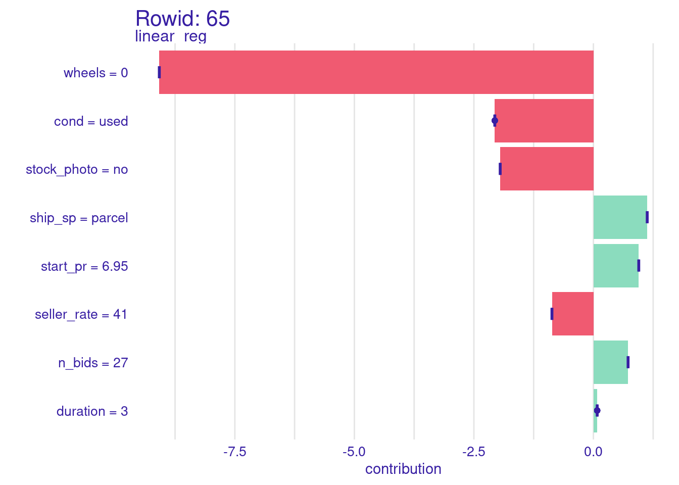
どちらもship_spがparcelですが、parcelだからといってすごく高額になるということはありません。titleから得られそうな情報に共通するものもなさそうなので、この元データだけからこれらの外れ値についてもうまく予測できるようにするのは難しそうです。
Discussion