カーネルSVMをシンプルに実装する


TL;DR
- 線形SVMと同様に、カーネルSVMを実装している記事もあまり見かけなかったのでpythonで実装してみました。
- カーネルSVMの主問題を、L2正則化経験リスク最小化問題として勾配降下法で解きます。
- 計算速度はscikit-learnのSVCのような工夫されたアルゴリズムには及びません。
本記事が実装するSVM
前回の線形SVMの記事はこちらです。
前回の線形SVMの内容を前提として進めたいと思います。
2クラス分類を行う、カーネルSVMの実装を行います。
実装はこちらにあります。
前回の記事の振り返り
線形SVM
ここで、線形分離不可能なデータセットに対して、
基本的なソフトマージンSVMは
主問題
定数
経験リスク最小化
線形SVMの主問題は経験リスク
線形SVMの限界
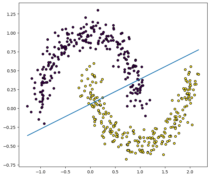
この線形SVMで、次のようなmoonデータセットを予測しようとすると、データセットの分布に沿った境界にはなっていません。
このように、上で扱った一次関数で分離するSVM(線形SVM)では限界があります。
カーネルSVMとは
特徴量
直感的には、データの特徴量を高次元に写すことで、表現力が増し、より分類しやすくなりそうです。しかし、特徴空間の次元が大きければ大きいほど、その空間での特徴量
ここで、特殊な関数であるカーネル関数
今回は、次のようにカーネル関数が表されるとします。
カーネルSVMの経験リスク関数
線形SVMの経験リスク
今、特徴量
このまま、前回の線形SVMと同様に勾配降下法を用いて解くことができればよいのですが、上で述べた通り、高次元空間での特徴量
ここで、一般的には双対問題を考えますが、今回は別の手法をとります。
この経験リスク
これを踏まえると経験リスク
ただし、
経験リスク
経験リスク最小化と最急降下法
線形SVMと同様に、経験リスク
つまり、
このステップを十分に繰り返すことで、重み
カーネルSVMでの予測
テストデータ
カーネルSVMの実装
ここでは、RBFカーネルを用いました。このカーネルにおける特徴写像
次のようにscikit-learnのAPIに寄せて実装しました。
import numpy as np


def _rbf_kernel(X: np.ndarray, Y: np.ndarray, gamma: float = 1.0):
    """Compute RBF kernel (Gaussian kernel).

    Parameters
    ----------
    X : numpy.ndarray
        First feature array.
    Y : numpy.ndarray
        Second feature array.
    gamma : float, default=1.0
        Parameter of the RBF kernel.

    Returns
    -------
    K : numpy.ndarray
        The RBF kernel.
    """
    # Compute the squared Euclidean distance between each pair of points in X and Y
    # ||x-y||^2 = ||x||^2 + ||y||^2 - 2 * x^T * y
    X_norm = np.sum(X**2, axis=1).reshape(-1, 1)
    Y_norm = np.sum(Y**2, axis=1).reshape(1, -1)
    D_square = X_norm + Y_norm - 2 * np.dot(X, Y.T)

    # Apply the RBF kernel formula
    K = np.exp(-gamma * D_square)

    return K


class KernelSVM:
    def __init__(
        self,
        lam: float = 0.01,
        n_iters: int = 5000,
        learning_rate: float = 0.01,
        kernel: str = "rbf",
        gamma: float = 1.0,
        bias=True,
        verbose=False,
    ):
        """Kernel Support Vector Machine (SVM) for Binary Classification.

        Parameters
        ----------
        lam : float, default=0.01
            Regularization parameter.
        n_iters : int, default=5000
            Number of iterations for the gradient descent.
        learning_rate : float, default=0.01
            Learning rate for the gradient descent.
        kernel : str, default="rbf"
            Kernel type to be used in the algorithm. It must be one of 'linear', 'rbf'.
        gamma : float, default=1.0
            Kernel parameter for 'rbf'.
        bias : bool, default=True
            Whether to include a bias term in the input matrix.
        verbose : bool, default=False
            If True, print progress messages during the gradient descent.
        """
        self.lam = lam
        self.n_iters = n_iters
        self.learning_rate = learning_rate
        self.bias = bias
        self.kernel = kernel
        self.gamma = gamma
        self.verbose = verbose
        self._Xfit = None
        self._classes = {}
        self._a = None

    # Calculate kernel function
    def _kernelize(self, X, Y):
        if self.kernel == "linear":
            return X @ Y.T
        elif self.kernel == "rbf":
            return _rbf_kernel(X, Y, gamma=self.gamma)
        else:
            raise ValueError(f"Unexpected kernel type: {self.kernel}")

    # Calculate the empirical risk function.
    def _empirical_risk(
        self, K: np.ndarray, y: np.ndarray, a_t: np.ndarray
    ) -> np.ndarray:
        regularzation = 0.5 * self.lam * (a_t @ K @ a_t)
        loss = np.where(1 - y * (K @ a_t) >= 0, 1 - y * (K @ a_t, 0)).mean()

        return regularzation + loss

    # Calculate the gradient of the empirical risk function.
    def _empirical_risk_grad(
        self, K: np.ndarray, y: np.ndarray, a_t: np.ndarray
    ) -> np.ndarray:
        regularzation_grad = self.lam * (K @ a_t)
        loss_grad = (
            (np.where(1 - y * (K @ a_t) >= 0, 1, 0) * -y).reshape(-1, 1) * K
        ).mean(axis=0)

        return regularzation_grad + loss_grad

    def fit(self, X: np.ndarray, y: np.ndarray):
        """Fit the Kernel SVM model according to the given training data.

        Parameters
        ----------
        X : numpy.ndarray of shape (n_samples, n_features)
            Training vectors, where `n_samples` is the number of samples
            and `n_features` is the number of features.

        y : numpy.ndarray of shape (n_samples,)
            Class labels in classification.

        Returns
        -------
        self : object
            Fitted estimator.
        """
        # validate and change class labels
        classes = np.unique(y)
        if len(classes) != 2:
            raise ValueError("Class labels is not binary")
        self._classes[-1] = classes[0]
        self._classes[1] = classes[1]
        y = np.where(y == self._classes[1], 1, -1)

        if self.bias:
            X = np.c_[X, np.ones(X.shape[0])]

        self._Xfit = X
        K = self._kernelize(X, X)

        # alpha for weights
        a = np.ones(K.shape[1])

        # gradient descent
        for i in range(self.n_iters):
            a = a - self.learning_rate * self._empirical_risk_grad(K, y, a)
            if self.verbose and (i + 1) % 1000 == 0:
                print(f"{i+1:4}: R(a) = {self._empirical_risk(K, y, a)}")
        self._a = a

    def decision_function(self, X: np.ndarray) -> np.ndarray:
        """Evaluate the decision function for the samples in X.

        Parameters
        ----------
        X : numpy.ndarray of shape (n_samples, n_features)
            The input samples.

        Returns
        -------
        y_score : ndarray of shape (n_samples, )
            Returns the decision function of the sample for each class in the model.
            The decision function is calculated based on the class labels 1 and -1.
        """
        if self.bias:
            X = np.c_[X, np.ones(X.shape[0])]

        K = self._kernelize(X, self._Xfit)
        y_score = K @ self._a

        return y_score

    def predict(self, X: np.ndarray) -> np.ndarray:
        """Perform classification on samples in X.

        Parameters
        ----------
        X : numpy.ndarray of shape (n_samples, n_features)

        Returns
        -------
        y_pred : ndarray of shape (n_samples,)
            Class labels for samples in X.
        """
        y_score = self.decision_function(X)
        y_pred = np.where(y_score > 0, 1, -1)
        y_pred = np.where(y_pred == 1, self._classes[1], self._classes[-1])

        return y_pred
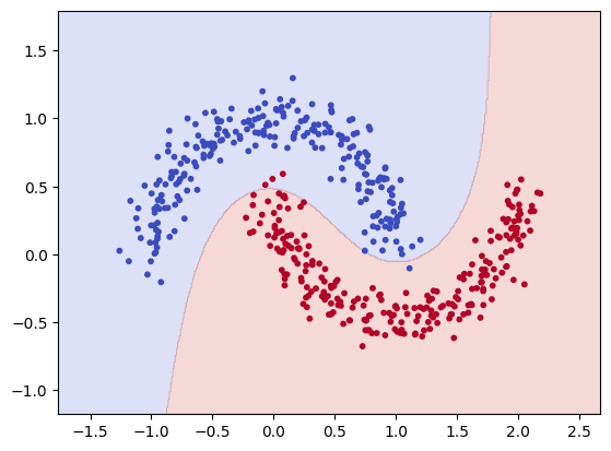
さて、このカーネルSVMをmoonデータセットに対して用いると次のようになります。
import numpy as np
from sklearn.datasets import make_moons
from sklearn.model_selection import train_test_split
from sklearn.metrics import accuracy_score
import matplotlib.pyplot as plt

np.random.seed(42)

X, y = make_moons(n_samples=500, noise=0.1, random_state=1)
X_train, X_test, y_train, y_test = train_test_split(X, y)

model = KernelSVM()
model.fit(X_train, y_train)
preds = model.predict(X_test)

print(f"ACC: {accuracy_score(y_test, preds)}")
#> ACC: 0.992

# Plot a decision boundary
x_min=X[:, 0].min() - 0.5
x_max=X[:, 0].max() + 0.5
y_min=X[:, 1].min() - 0.5
y_max=X[:, 1].max() + 0.5

xx, yy = np.meshgrid(np.arange(x_min, x_max, 0.01), np.arange(y_min, y_max, 0.01))
XY = np.array([xx.ravel(), yy.ravel()]).T
z = model.predict(XY)
plt.contourf(xx, yy, z.reshape(xx.shape), alpha=0.2, cmap=plt.cm.coolwarm)
plt.scatter(X[:, 0], X[:, 1], c=y, s=10, cmap=plt.cm.coolwarm)
plt.show()
ACCは0.992となり、識別境界もデータセットに合った形となっています。
Discussion