RNNの共和分法への応用~株価ポートフォリオ価値の取引シミュレーション
概要
株価がいくらになるかという回帰型の予測問題を考え、
この予測結果を統計的裁定に応用する方法を検討してみます。
定常性のないデータの予測は難しいので、定常性は確保しておきたいです。
そこで、共和分検定にパスした共和分過程とみなせる銘柄の組み合わせを扱うことにします。
こうすることによって、統計的裁定の一つである共和分法へも応用しやすくなります。
取引シミュレーションには、RNNを用いたポートフォリオ価値の予測器を使います。
RNNはディープラーニングの中でも、系列データの予測に特化したアーキテクチャです。
検証環境
Google Colaboratory
2022年3月11日
データ取得
ライブラリのインポート
まずは、必要なライブラリをインポートします。
from datetime import date

import matplotlib
import matplotlib.pyplot as plt

import sklearn
import sklearn.model_selection

import pandas as pd
import numpy as np

import warnings
warnings.filterwarnings('ignore')

!pip install yfinance

from pandas_datareader import data as pdr

import yfinance as yf
yf.pdr_override()
S&P500採用銘柄を取得します。
url = "https://raw.githubusercontent.com/datasets/s-and-p-500-companies/master/data/constituents.csv"
codelist = pd.read_csv(url, encoding="SHIFT_JIS")
codelist['Sector'].unique()
S&P500採用銘柄のセクターが出力されます。
array(['Industrial Conglomerates', 'Building Products',
       'Health Care Equipment', 'Pharmaceuticals',
       'IT Consulting & Other Services', 'Interactive Home Entertainment',
       'Agricultural Products', 'Application Software',
       ・・・・・,
       'Trading Companies & Distributors', 'Drug Retail', 'Broadcasting',
       'Household Appliances'], dtype=object)
今回はS&P500採用銘柄のうちIT関連企業に属するものに絞って、データを用意します。
セクター名に変更があった場合や、他のセクターで試したい場合は
sectorsの中身を適宜変更してください。
# Information Technology
sectors = ['IT Consulting & Other Services', 'Application Software', 'Technology Hardware, Storage & Peripherals']
symbols = codelist[codelist['Sector'].isin(sectors)]['Symbol'].unique()
symbols
array(['ACN', 'ADBE', 'ANSS', 'AAPL', 'ADSK', 'CDNS', 'CDAY', 'CTSH',
       'DXC', 'EPAM', 'IT', 'GEN', 'HPE', 'HPQ', 'IBM', 'INTU', 'NTAP',
       'ORCL', 'PAYC', 'PTC', 'CRM', 'STX', 'SNPS', 'TYL', 'WDC'],
      dtype=object)
データを準備します。
start = '2015-01-01'
end = date.today().strftime('%Y-%m-%d')

df = pd.DataFrame()
for symbol in symbols:
    print(symbol)
    data = pdr.get_data_yahoo(symbol,start,end)['Adj Close']
    data.name = symbol
    df = pd.concat([df,data],axis = 1)

for i in np.arange(len(df.index)):
    df.index.values[i] = str(df.index[i].date())

df.index = df.index.rename('Date')
学習に使う訓練データとテスト・データに分割します。
ここで、検証データではなくテスト・データという名前を使っていることに注意してください。
訓練データに共和分検定を行った後、さらに訓練データの中から検証データを取り分けます。
この検証データを用いて、取引シミュレーションに必要なハイパーパラメータを決めます。
テスト・データは最終的なモデルの性能の確認まで取っておく必要があります。
from sklearn.model_selection import train_test_split

test_size = 0.2
df_train, df_test = train_test_split(df,test_size = test_size,shuffle = False)

test_num = len(df_test)
共和分検定
上記の手順で得られた訓練データに共和分検定を行い、ポートフォリオの銘柄を選択します。
ただし、本記事では、シンプルなペアトレーディングを扱うのみにします。
import itertools
# Johansen procedure
from statsmodels.tsa.vector_ar.vecm import coint_johansen

pairs = []
i = 1
for comb in itertools.combinations(df_train.columns,2):
    prices = df_train.loc[:,comb]
    prices = prices.dropna()
    try:
        # JohansenTestResult
        jrt = coint_johansen(prices,k_ar_diff=0,det_order=-1)
        if jrt.lr1[0] > jrt.cvt[0,2] and jrt.lr1[1] < jrt.cvt[1,0]\
        and jrt.lr2[0] > jrt.cvm[0,2] and jrt.lr2[1] < jrt.cvm[1,0]:
            pairs.append(comb)
    except ValueError as error:
        print(i,comb)
    i += 1

print(pairs)
print(len(pairs))
[('ACN', 'AAPL'), ('ACN', 'CDNS'), ('ACN', 'CTSH'), ('ACN', 'EPAM'), ('ACN', 'SNPS'),・・・, ('IBM', 'INTU'), ('IBM', 'ORCL'), ('INTU', 'ORCL')]
36
itertoolsパッケージに含まれるcombinations()を使い、
組み合わせを列挙しています。
3銘柄の組み合わせをつくりたい場合は、
combinations()の第2引数を2から3にしてください。
try節の中身について
coint_johansen(prices,k_ar_diff=0,det_order=-1):共和分検定を行う。
k_ar_diffは差分の次数、det_orderは定数項やトレンド項の有無を指定
jrt.lr1[0]:trace testの最初の統計量、つまりΠのランクが0であるとい帰無仮説に対する統計量
jrt.cvt[0,2]:上記の帰無仮説に対する99%棄却限界値
jrt.lr1[0] > jrt.cvt[0,2]が成り立つとき、
ペアは共和分ベクトルを少なくとも1つは持つと、
trace testからはいえることになります。
jrt.lr1[1]:trace testにおいて、Πのランクが1であるとい帰無仮説に対する統計量
jrt.cvt[1,0]:上記の帰無仮説に対する90%棄却限界値
jrt.lr1[1] < jrt.cvt[1,0]が成り立つとき、帰無仮説は棄却できません。
もし棄却されたら、Πのランクは2になりますが、
今回のように2組の銘柄の組み合わせを考えている場合、
Πは2×2行列なので、共和分ベクトルで結合するまでもなく、
定常性が担保されてしまいます。
その場合は、共和分ベクトルに対して適用するVECMモデルではなく、
定常過程に適用するVARモデルなどを使うことになると思います。
しかし、本記事では、共和分法を利用したいため、ランクが1の場合を探索します。
次の行のjrt.lr2[0] > jrt.cvm[0,2] and jrt.lr2[1] < jrt.cvm[1,0]
も同じようなことをmax test(最大固有値)に対して行っています。
帰無仮説の立て方が違うだけで、trace testと同じようなことをやっています。
この作業によって、36組まで絞れました。
共和分を持つペアが見つかっても、
それがたまたま共和分をもつように見えただけかもしれないので、
他の方法でも確認をしておきます。
本記事では、
実際にポートフォリオを組んでみた場合のペア価格の変動が定常性をもっているかを
Hurst exponentを計算することで確認します。
統計量Hが0.5より小さい、すなわち平均回帰性を持つペアを採用します。
!pip install hurst # https://pypi.org/project/hurst/
from hurst import compute_Hc

from statsmodels.tsa.vector_ar.vecm import VECM
pairs2 = []

for i in range(len(pairs)):
    # modelpair = df_train[[pairs[i][0], pairs[i][1]]].replace(0, np.nan)
    modelpair = df_train[[pairs[i][0], pairs[i][1]]].dropna()
    modelCoint = VECM(modelpair,k_ar_diff=0,deterministic='na')
    res = modelCoint.fit()

    # 得られた係数をもとにペアー価値の時系列を構成する
    portfolio = res.beta[0]*df_train[pairs[i][0]] + res.beta[1]*df_train[pairs[i][1]]
    # portfolio = portfolio.replace(0, np.nan)
    portfolio = portfolio.dropna()
    # ポートフォリオ価値時系列データに対してhurst.compute_Hc関数を適用してHurst exponent(H)とその信頼区間(c)およびデータサイズ(data_size)を求める
    H, c, data_size = compute_Hc(portfolio) # Hurst exponent計算

    if H < 0.5: # 0 < H < 0.5 — anti-persistent behavior.
        pairs2.append((pairs[i][0], pairs[i][1]))
    i += 1

print(pairs2)
print(len(pairs2))
実際にポートフォリオを組んでみた場合のペア価格の変動が
定常性をもっているかを確認する方法としては、
他には結果の可視化やサンプルを入れ替えて検定を行う交差検証などが考えられます。
ポートフォリオ価値の構成
以下の実装では、(HPQ,PTC)を採用します。
HPQとは
HPQ(ヒューレット・パッカード)は米国大手のコンピュータ・IT企業です。
「HP」ブランドを展開、デスクトップ型またはノートブック型パソコン、
インクまたはレーザープリンター、スキャナーなどを開発、製造、販売している企業です。
PTCとは
PTCは米国のソフトウェア会社です。
主要ソフトウェア製品はコンピュータ支援設計(CAD)、製品ライフサイクル管理(PLM)、
アプリケーションライフサイクル管理(ALM)、サプライチェーン管理(SCM)、
サービスライフサイクル管理(SLM)などです。
また、ソフトウェアのライセンス供与、サポート、サービスも提供している企業です。
# 共和分検定をパスした共和分ペアを使ってモデルを構成する
from statsmodels.tsa.vector_ar.vecm import VECM
pair = ['HPQ','PTC']

modelCoint = VECM(df_train[pair],k_ar_diff=0,deterministic='na',coint_rank = 1) # coint_rank = 1 は省略可
res = modelCoint.fit()

# 得られた係数をもとにペアー価値の時系列を構成する
pairs_value = res.beta[0]*df[pair[0]] + res.beta[1]*df[pair[1]]
plt.plot(pairs_value)

RNNのためのデータ整理
ここでは、一つ一つの系列の長さが70になるように、
これまでに構成したポートフォリオの価値のデータを変換していきます。
ある日付から1日前のポートフォリオ価値から70日前のポートフォリオ価値までを
まとめて一つのデータにします。
serlen = 70

df_ser = pd.DataFrame()
columns = []
for i in range(serlen + 1):
    df_ser = pd.concat([df_ser,pairs_value.shift(i)],axis = 1)
    columns.append('{} day shift'.format(i))
df_ser.columns = columns
df_ser = df_ser.dropna()

X = df_ser.loc[:,'1 day shift':]
y = df_ser['0 day shift']
上記のように、データをターゲットと特徴量に分割したのち、
改めてテスト・データを取り分けます。
テスト・データは予め保存していたデータ数(test_num)だけ取り分けます。
train_size = 0.8

X_train,X_test,y_train,y_test= train_test_split(X,y,
                                                test_size = test_num,
                                                shuffle = False)
X_train,X_val,y_train,y_val = train_test_split(X_train,y_train,
                                               train_size = train_size,
                                               shuffle = False)

val_num = y_val.shape[0]
RNN
ここからは、RNNを実装していきます。
そのためにデータを変換します。
X_train_values = X_train.values.reshape(-1,serlen,1)
X_val_values = X_val.values.reshape(-1,serlen,1)
X_test_values = X_test.values.reshape(-1,serlen,1)
y_train_values = y_train.values.reshape(-1,1)
y_val_values = y_val.values.reshape(-1,1)
y_test_values = y_test.values.reshape(-1,1)
特徴量は3階のテンソル(3つの要素を持った数の組み合わせ)になっています。
上記のコードで、reshape(-1,serlen,1)とある箇所の
1つ目の引数にはデータ数、2つ目の引数にはタイムステップ(系列を遡る数)、
3つ目の引数には特徴量の数を指定します。
今回は、過去から現在までのポートフォリオ価値のみを使って予測するので特徴量は1つですが、
為替レートなど複数種類のファクターを加えて予測するのであれば、
最後の引数には1以上の数が与えられます。
同様に予測のターゲットが次の時点のポートフォリオ価値以外のものを考えなければならないとき、y_train.values.reshape(-1,1)の2つ目の引数も1以上の数があてられます。
RNNを実装するために必要なパッケージをインポートします。
import tensorflow as tf
from tensorflow.keras.models import Sequential
from tensorflow.keras.layers import Dense, SimpleRNN
from tensorflow.keras import optimizers
from tensorflow.keras.callbacks import EarlyStopping
次にRNNで学習します。
隠れ層のユニットは70、早期終了を設定した上で、optimizerにはRMSpropを使います。
tf.random.set_seed(321)
modelRNN = Sequential()
modelRNN.add(SimpleRNN(70, activation = 'tanh'))
modelRNN.add(Dense(1,activation = 'linear'))
optimizer = optimizers.RMSprop(learning_rate = 0.001,rho=0.99)
modelRNN.compile(optimizer = optimizer, loss = 'mean_squared_error')
es = EarlyStopping(monitor = 'loss',
patience = 5,
verbose = 1)
modelRNN.fit(X_train_values,y_train_values,
epochs = 10000, batch_size = 10,verbose = 1,
callbacks = [es],
validation_data = (X_val_values,y_val_values))
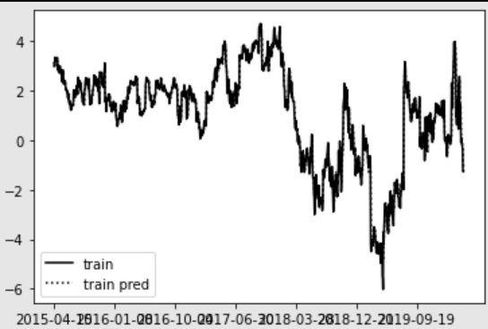
y_train_pred = modelRNN.predict(X_train_values).reshape(-1,)
y_val_pred = modelRNN.predict(X_val_values).reshape(-1,)
予測値は、modelRNN.predict()で出力できますが、
中身はテンソルの形式になっていて分かりにくいので、
reshape(-1,)としてベクトルに変換してから図示します。
fig1 = plt.figure()
plt.plot(y_train.index, y_train,
         label = 'train',
         color = 'black',
         linestyle = 'solid')
plt.plot(y_train.index, y_train_pred,
         label= 'train pred',
         color = 'black',
         linestyle = 'dotted')
plt.xticks(y_train.index[np.arange(0,len(y_train.index)+1,186)])
plt.legend()
fig2 = plt.figure()
plt.plot(y_val.index, y_val,
         label = 'val',
         color = 'black',
         linestyle = 'solid')
plt.plot(y_val.index, y_val_pred,
         label = 'val pred',
         color = 'black',
         linestyle = 'dotted')
plt.xticks(y_val.index[np.arange(0,len(y_val.index)+1,46)])
plt.legend()


今回は、将来のポートフォリオ価値の値を予測する問題であり、
隠れ層から出力層に投げ込まれた値を線形変換したものが出力になります。
なので、出力層での活性化関数は線形とし、誤差の尺度も平均二乗誤差とします。
from sklearn.metrics import r2_score

print('R score, RNN',r2_score(y_val,y_val_pred))
R score, RNN -0.9942877837714026
LSTM
RNNは長期の時間依存に対して勾配消失問題を起こしやすい、
つまり古い情報を忘れてしまうという欠点がありました。
このようなRNNが持つ問題に対処するために、
シンプルなRNNを拡張したLSTMというアーキテクチャを試してみます。
from tensorflow.keras.layers import LSTM
隠れ層のユニットは70、早期終了を設定した上で、optimizerにはAdamを使います。
tf.random.set_seed(123)
tf.random.set_seed(321)

modelLSTM = Sequential()
modelLSTM.add(LSTM(70, activation = 'tanh'))
modelLSTM.add(Dense(1,activation = 'linear'))
optimizer = optimizers.Adam(learning_rate = 0.01,
                            beta_1 = 0.9,
                            beta_2 = 0.999,
                            amsgrad = True)
modelLSTM.compile(optimizer = optimizer, loss = 'mean_squared_error')
es = EarlyStopping(monitor = 'loss',
                  patience = 5,
                  verbose = 1)
modelLSTM.fit(X_train_values,y_train_values,
         epochs = 100, batch_size = 10,verbose = 1,
         callbacks = [es],
         validation_data = (X_val_values,y_val_values))
y_train_pred = modelLSTM.predict(X_train_values).reshape(-1,)
y_val_pred = modelLSTM.predict(X_val_values).reshape(-1,)
fig3 = plt.figure()
plt.plot(y_train.index,y_train,label = 'train',
         color = 'black',
         linestyle = 'solid')
plt.plot(y_train.index, y_train_pred,
         label= 'train pred',
         color = 'black',
         linestyle = 'dotted')
plt.xticks(y_train.index[np.arange(0,len(y_train.index)+1,186)])
plt.legend()
fig4 = plt.figure()
plt.plot(y_val.index,y_val,
         label = 'val',
         color = 'black',
         linestyle = 'solid')
plt.plot(y_val.index, y_val_pred,
         label = 'val pred',
         color = 'black',
         linestyle = 'dotted')
plt.xticks(y_val.index[np.arange(0,len(y_val.index)+1,46)])
plt.legend()

print('R score, LSTM',r2_score(y_val,y_val_pred))
R score, LSTM 0.695658330013414
RNNの時と比較したら結果は良くなりました。
GRU
次に、LSTMを簡略化したGRU(gatad recurrent unit)を試してみます。
from tensorflow.keras.layers import GRU

tf.random.set_seed(123)
modelGRU = Sequential()
modelGRU.add(GRU(70, activation = 'tanh'))
modelGRU.add(Dense(1,activation = 'linear'))
optimizer = optimizers.Adam(learning_rate = 0.01,
                            beta_1 = 0.9,
                            beta_2 = 0.999,
                            amsgrad = True)
modelGRU.compile(optimizer = optimizer, loss = 'mean_squared_error')
es = EarlyStopping(monitor = 'loss',
                  patience = 5,
                  verbose = 1)
modelGRU.fit(X_train_values,y_train_values,
         epochs = 100, batch_size = 10,verbose = 1,
         callbacks = [es],
         validation_data = (X_val_values,y_val_values))

print(len(modelGRU.predict(X_val_values)))
print(len(y_val_values))
316
316
y_train_pred = modelGRU.predict(X_train_values).reshape(-1,)
y_val_pred = modelGRU.predict(X_val_values).reshape(-1,)
fig5 = plt.figure()
plt.plot(y_train.index,y_train,label = 'train',color = 'black',linestyle = 'solid')
plt.plot(y_train.index, y_train_pred,
         label= 'train pred',
         color = 'black',
         linestyle = 'dotted')
plt.xticks(y_train.index[np.arange(0,len(y_train.index)+1,186)])
plt.legend()


fig6 = plt.figure()
plt.plot(y_val.index, y_val,
         label = 'val',
         color = 'black',
         linestyle = 'solid')
plt.plot(y_val.index, y_val_pred,
         label = 'val pred',
         color = 'black',
         linestyle = 'dotted')
plt.xticks(y_val.index[np.arange(0,len(y_val.index)+1,46)])
plt.legend()


print('R score, GRU',r2_score(y_val,y_val_pred))
R score, GRU 0.35416359216078375
LSTMの時と比べたら、精度は落ちましたが、それでも、
シンプルなRNNと比べたらかなりの精度がでています。
取引シミュレーション
共和分法はポートフォリオの構成までは決めてくれますが、
どのタイミングでポジションを取るべきで、
どのタイミングでポジションを解消するべきかまでは分かりません。
共和分法は、ポートフォリオがやがて収束するであろう回帰水準を示してくれるので、
回帰水準から最も離れたときにポジションをとり、
回帰水準に収束したタイミングでポジションを解消するのが理想的です。
しかし、この場合でも回帰水準から最も離れた時はいつなのかという疑問が残ります。
標準偏差の2倍を超えた時にポジションを取るような手法もありますが、
今回は以下を参考にして次のような投資戦略を試してみます。
1.閾値の計算
2.ポートフォリオ価値の変動を予測
3.ポジションがない場合は、予測変動が閾値を超えた時にポジションをとる
ポジションがある場合は、予測変動の符号が反転するまでポジションを持ち続け、
反転したら解消
閾値の決め方としては、
訓練期間のポートフォリオ価値の変動の標準偏差を利用することなどが考えられますが、
今回は参考元にならい、分位点を使います。
分位点の取り方にも様々な選択がありますが、5分位点と10分位点を候補とします。
そして、どちらがよいか、データを使って以下の手順で検証します。
1.訓練データでポートフォリオ価値の変動の上下10%点と20%点を計算
2.検証データで10%点を閾値として計算した取引収益と、
20%点を閾値として計算した取引収益を比較して、より高い収益をもたらす閾値を採用
閾値の候補
まず、ポートフォリオ価値の上下10%点と20%点を計算します。
diff = (y_train.shift(-1) - y_train).dropna()
diff_p = diff[diff > 0] # 正の変動を格納
diff_m = diff[diff <= 0] # 負の変動を格納

quintile_range = (diff_m.quantile(0.2),diff_p.quantile(0.8)) # 上位20%,下位20%から5分位点を作る
decile_range = (diff_m.quantile(0.1),diff_p.quantile(0.9)) # 上位10%,下位10%から10分位点を作る

print('quintile threshold',quintile_range)
print('decile threshold',decile_range)
quintile threshold (-0.30606302532491725, 0.31557066224317376)
decile threshold (-0.4639020518585788, 0.46598918933239847)
予測値の格納
次に検証期間とテスト期間の予測値を計算し、その変動の予測値を記憶しておきます。
y_val_pred = modelGRU.predict(X_val_values).reshape(-1,)
y_test_pred = modelGRU.predict(X_test_values).reshape(-1,)

diff_val = (y_val_pred[1:] - y_val[:-1])
diff_test = (y_test_pred[1:] - y_test[:-1])
それでは、検証期間における収益を計算します。
検証データを使って5分位点のシミュレーション
pos_q = 0 # 0 no position, 1 long positon, -1 short position
port_val_q = 0.0

# 5分位点の閾値検証
for i,diff in enumerate(diff_val[:-1]): # 投資期間終了の直前までループ
    index = diff_val.index[i]
    if pos_q == 0:
        if diff > quintile_range[1]: # ロング・ポジションを組む
            pos_q = 1
            ini_val_q = pairs_value[index]
            print('long position is made at', index,
                  'by the value of ',pairs_value[index])
        elif diff < quintile_range[0]: # ショート・ポジションを組む
            pos_q = -1
            ini_val_q = pairs_value[index]
            print('short position is made at', index,
                  'by the value of', pairs_value[index])
    #符号が反転したら利益を確定
    elif pos_q == 1 and diff < 0: # ロング・ポジションの利益確定
        port_val_q += (pairs_value[index] - ini_val_q)
        pos_q = 0 # ポジションを解消する
        print('long position is liquidated at',index,
              'current portfolio value is', port_val_q,
              'current pair value is', pairs_value[index])
    elif pos_q == -1 and diff > 0:# ショートポジションの利益確定
        port_val_q -= (pairs_value[index] - ini_val_q)
        pos_q = 0 # ポジションを解消する
        print('short position is liquidated at',index,
              'current portfolio value is', port_val_q,
              'current pair value is', pairs_value[index])

# 満期にポジションは強制終了
index = diff_val.index[-1]
if pos_q == 1:# ロング・ポジションの利益確定
    port_val_q += (pairs_value[index] - ini_val_q)
    print('long position is liquidated at',index,
          'current portfolio value is', port_val_q)
if pos_q == -1:# ショート・ポジションの利益確定
    port_val_q -= (pairs_value[index] - ini_val_q)
    print('short position is liquidated at',index,
          'current portfolio value is', port_val_q)

print(port_val_q)
long position is made at 2020-05-05 by the value of  -2.739433524789767
long position is liquidated at 2020-05-15 current portfolio value is 1.2728604147335627 current pair value is -1.4665731100562045
long position is made at 2020-05-28 by the value of  -3.613964746406488
long position is liquidated at 2020-06-26 current portfolio value is 2.7321325595988224 current pair value is -2.154692601541228
long position is made at 2020-07-09 by the value of  -4.523318453029855
long position is liquidated at 2020-07-13 current portfolio value is 4.909948721551272 current pair value is -2.3455022910774055
short position is made at 2020-07-14 by the value of -1.7342950577129912
short position is liquidated at 2020-07-20 current portfolio value is 6.104502289151489 current pair value is -2.9288486253132078
short position is made at 2020-10-05 by the value of -1.1672449643724754
short position is liquidated at 2020-10-23 current portfolio value is 7.787275901128696 current pair value is -2.850018576349683
long position is made at 2020-12-21 by the value of  -5.264656062609792
long position is liquidated at 2021-03-02 current portfolio value is 9.661084249791164 current pair value is -3.3908477139473234
short position is made at 2021-03-05 by the value of -1.1244126181674403
short position is liquidated at 2021-03-11 current portfolio value is 11.308545758048604 current pair value is -2.77187412642488
short position is made at 2021-03-17 by the value of -1.562415731031642
short position is liquidated at 2021-04-01 current portfolio value is 12.760489303120218 current pair value is -3.0143592761032565
short position is made at 2021-04-19 by the value of -0.5218310293950026
short position is liquidated at 2021-04-30 current portfolio value is 10.330428587296309 current pair value is 1.908229686428907
long position is made at 2021-05-28 by the value of  -3.424807986101989
long position is liquidated at 2021-07-19 current portfolio value is 8.359390813488618
8.359390813488618
検証データを使って10分位点のシミュレーション
# 10分位点の閾値検証
pos_d = 0
port_val_d = 0.0

#trade_count = 0
for i,diff in enumerate(diff_val[:-1]):
    index = diff_val.index[i]
    if pos_d == 0:
        if diff > decile_range[1]: # ロング・ポジションを組む
            pos_d = 1
            ini_val_d = pairs_value[index]
            print('long position is made at', index,
                  'by the value of ',pairs_value[index])

        elif diff < decile_range[0]: # ショート・ポジションを組む
            pos_d = -1
            ini_val_d = pairs_value[index]
            print('short position is made at', index,
                  'by the value of', pairs_value[index])
    #符号が反転したら利益を確定
    elif pos_d == 1 and diff < 0: # ロング・ポジションの利益確定
        port_val_d += (pairs_value[index] - ini_val_d)
        pos_d = 0 # ポジションを解消する
        print('long position is liquidated at', index,
              'current value is', pairs_value[index])
    elif pos_d == -1 and diff > 0:# ショートポジションの利益確定
        port_val_d -= (pairs_value[index] - ini_val_d)
        pos_d = 0 # ポジションを解消する
        print('short position is liquidated at', index,
              'current value is', pairs_value[index])

# 満期にポジションは強制終了
```py:Python
index = diff_val.index[-1]
if pos_d == 1:# ロング・ポジションの解消
    port_val_d += (pairs_value[index] - ini_val_d)
    print('long position is liquidated at', index,
          'current value is', port_val_d)
if pos_d == -1:# ショート・ポジションの利益確定
    port_val_d -= (pairs_value[index] - ini_val_d)
    print('short position is liquidated at', index,
          'current value is', port_val_d)

print(port_val_d)
long position is made at 2020-05-05 by the value of  -2.739433524789767
long position is liquidated at 2020-05-15 current value is -1.4665731100562045
long position is made at 2020-05-28 by the value of  -3.613964746406488
long position is liquidated at 2020-06-26 current value is -2.154692601541228
long position is made at 2020-12-21 by the value of  -5.264656062609792
long position is liquidated at 2021-03-02 current value is -3.3908477139473234
long position is made at 2021-05-28 by the value of  -3.424807986101989
long position is liquidated at 2021-07-19 current value is 2.6349031344536
2.6349031344536
5分位点と10分位点のシミュレーション結果比較
print((port_val_q,port_val_d))
(8.359390813488618, 2.6349031344536)
if port_val_q > port_val_d:
    threshold = quintile_range
else:
    threshold = decile_range

print('optimal threshold is', threshold)
optimal threshold is (-0.30606302532491725, 0.31557066224317376)
テストデータを用いた取引シミュレーション
pos = 0 # 0 for no position, 1 for long positon, -1 for short position
port_val = 0.0
port_hist = pd.DataFrame()

for i,diff in enumerate(diff_test[:-1]):
    index = diff_test.index[i]
    if pos == 0:
        if diff > threshold[1]: # ロング・ポジションを組む
            pos = 1
            ini_val = pairs_value[index]
            print('long position is made at', index,
                  'by the value of ',pairs_value[index])
        elif diff < threshold[0]: # ショート・ポジションを組む
            pos = -1
            ini_val = pairs_value[index]
            print('short position is made at', index,
                  'by the value of', pairs_value[index])
    #符号が反転したら利益を確定
    if pos == 1 and np.sign(diff) < 0: # ロング・ポジションの利益確定
        port_val += (pairs_value[index] - ini_val)
        pos = 0 # ポジションを解消する
        print('long position is liquidated at', index,
              'current value is', pairs_value[index])
    if pos == -1 and np.sign(diff) >= 0:# ショートポジションの利益確定
        port_val -= (pairs_value[index] - ini_val)
        pos = 0 # ポジションを解消する
        print('short position is liquidated at', index,
              'current value is', pairs_value[index])
    ser = pd.DataFrame([pos],index = [index])
    port_hist = port_hist.append(ser)


# 満期にポジションは強制終了
index = diff_test.index[-1]
if pos == 1:# ロング・ポジションの利益確定
    port_val += (pairs_value[index] - ini_val)
    print('long position is liquidated at', index,
          'current value is', pairs_value[index])
if pos == -1:# ショート・ポジションの利益確定
    port_val -= (pairs_value[index] - ini_val)
    print('short position is liquidated at', index,
          'current value is', pairs_value[index])
ser = pd.DataFrame([pos],index = [index])
port_hist = port_hist.append(ser)

print('Portfolio value is', port_val)
long position is made at 2021-07-21 by the value of  -6.773183507750119
long position is liquidated at 2021-08-17 current value is -2.3489576098386777
short position is made at 2021-09-13 by the value of -1.2646347279476657
short position is liquidated at 2021-10-13 current value is -2.5854046704389013
short position is made at 2021-10-21 by the value of -0.3709224126325701
short position is liquidated at 2021-11-05 current value is 1.4182174709943425
short position is made at 2021-11-23 by the value of 5.389123351879459
short position is liquidated at 2022-08-31 current value is 1.4352992088706813
long position is made at 2022-09-01 by the value of  0.9005391179624702
long position is liquidated at 2022-10-19 current value is -0.032465583841911894
long position is made at 2022-11-03 by the value of  -2.240464356067463
long position is liquidated at 2022-11-08 current value is -0.6162913008405653
long position is made at 2022-11-09 by the value of  -1.7348661580645732
long position is liquidated at 2022-11-11 current value is -0.4398539707256752
long position is made at 2022-11-16 by the value of  -1.1947713637442625
long position is liquidated at 2022-11-17 current value is 0.31767193492174783
short position is made at 2022-11-30 by the value of 0.1460329907772504
short position is liquidated at 2023-01-23 current value is -2.8035359008177743
short position is made at 2023-02-02 by the value of -0.017718154669353225
short position is liquidated at 2023-03-09 current value is 0.0764737162994038
Portfolio value is 14.263680959838233
fig8 = plt.figure()

ax1 = fig8.add_subplot(211)
ax1.plot(pairs_value[diff_test.index].index,
         pairs_value[diff_test.index].values,
         color='black',
         label='Pairs value')
ax1.set_xticks(pairs_value[diff_test.index].index[::50])
ax1.legend()

ax2 = fig8.add_subplot(212)
ax2.plot(port_hist.index,
         port_hist.values,
         color='black',
         label = 'Position')
ax2.set_yticks([-1,0,1])
ax2.set_xticks(port_hist.index[::50])
ax2.legend()
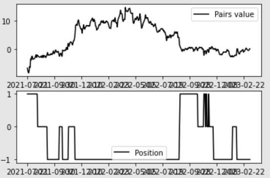
最終的に約14の利益を得ることができました。
しかし、今回のペアトレードでは、ロングとショートの組み合わせで
取引コストがかさみやすいため、ここから取引コストを差し引いて評価すべき
ことには注意が必要です。
参考文献
・吉川大介, データ駆動型ファイナンス ー基礎学習からPython機械学習による応用ー, 2022年, 共立出版
Discussion