時系列の予測モデルを比較してみた
2021/9/24 salesforce の Merlionについて追記
2021/10/9 TimeSeriesSplit(), PytorchのLSTMについて続編を書いた
時系列データの予測モデルである、Prophet、sktime、LSTM と lightGBMを使った時系列予測を比較してみました。
コードはGoogle Colabがこちら、GitHubがこちら。
ただし途中のグラフで使用しているドロップボックスについては Google Colab 専用の機能になりますのでご留意ください。
細かいコードは割愛しています。
Google Colabでドロップボックス等の機能を使う方法についてはこちら。
なお、使っているデータセットはアメリカンフットボールプレーヤのPayton ManningのWikiアクセス数のデータだそうです。
Merlion
Merlion は Salesforce の時系列予測、異常検知用のライブラリです。
from merlion.utils import TimeSeries
from merlion.models.defaults import DefaultForecasterConfig, DefaultForecaster

model = DefaultForecaster(DefaultForecasterConfig())

# データ変換
train_ts = TimeSeries.from_pd(train.set_index("ds"))
test_ts = TimeSeries.from_pd(test.set_index("ds"))

# 学習
model.train(train_data=train_ts)

# 予測データの作成
pred_merlion, test_err_merlion = model.forecast(time_stamps=test_ts.time_stamps)

pred_merlion.to_pd().head()
ちなみに公式リポジトリに書いてあるやり方と違うが、以下のやり方で公式リポジトリに入っているデータセットを使うことができた。
!git clone https://github.com/salesforce/Merlion

# 参考 datasets の使用
import sys
sys.path.append("/content/Merlion/ts_datasets")

from ts_datasets.forecast import M4

# Data loader returns pandas DataFrames, which we convert to Merlion TimeSeries
time_series, metadata = M4(subset="Hourly")[0]
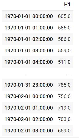
timeseries型という特殊?な型に変換するようだが、.to_pd()でDataFrame型に変換できるし、.time_stamps で index の時系列カラムを取得できるようです。
Prophet
Prophet はフェイスブック製の時系列用フレームワークで、日付データのカラム名を ds 、目的変数のカラム名を y とする必要があるのでやや癖があります。
またインストールが難しく、Anaconda を使っている場合は conda 経由でインストールするのが無難と思われます。
from fbprophet import Prophet

# モデルの作成
model = Prophet(weekly_seasonality=True, yearly_seasonality=True, daily_seasonality=True)

# 学習
model.fit(train)

# 予測データの作成
pred = model.predict(test)
sktime
sktimeも時系列用のフレームワークでです。
また、時系列向けの学習データ、訓練データの分割ライブラリもあります。
スライス指定しなくてもいいのでちょっと便利です。
from sktime.forecasting.model_selection import temporal_train_test_split
train, test = temporal_train_test_split(df, test_size=365)
from sktime.forecasting.all import *

# 日時データをindexに変換
train_sk = train.set_index("ds")
test_sk = test.set_index("ds")

# 学習
model = ThetaForecaster(sp=365)
model.fit(train["y"])

fh = ForecastingHorizon(test.index, is_relative=False)

# 予測データの作成
pred_sktime = model.predict(fh)
LSTM
LSTM は時系列や自然言語処理に向いたニューラルネットワークです。
なお、LSTM は Long Short Term Memory の略だそうです。
後ほど紹介するlightGBMで時系列解析する場合のラグ作成に近いですが、目的変数から特徴量を作成する必要があるようです。
詳細はこちらの記事をご参照ください。
import keras
from keras.models import Sequential
from keras.layers import Dense, Activation, LSTM
from keras.optimizers import Adam
import tensorflow as tf

# 目的変数と説明変数の作成
def make_dataset(low_data, maxlen):

    data, target = [], []

    for i in range(len(low_data)-maxlen):
        data.append(low_data[i:i + maxlen])
        target.append(low_data[i + maxlen])

    re_data = np.array(data).reshape(len(data), maxlen, 1)
    re_target = np.array(target).reshape(len(data), 1)

    return re_data, re_target

# RNNへの入力データ数
window_size = 12

# 入力データと教師データへの分割
X, y = make_dataset(df["y"], window_size)

# データの分割
X_train, X_test, y_train, y_test = temporal_train_test_split(X, y, test_size=365)

# バリデーションデータの作成
X_train, X_val, y_train, y_val = temporal_train_test_split(X_train, y_train, test_size=365)
# ネットワークの構築
model = Sequential() # Sequentialモデル

model.add(LSTM(50, batch_input_shape=(None, window_size, 1))) # LSTM 50層
model.add(Dense(1)) # 出力次元数は1

#コンパイル
model.compile(loss='mean_squared_error', optimizer=Adam() , metrics = ['accuracy'])
model.summary()
Model: "sequential_1"
_________________________________________________________________
Layer (type)                 Output Shape              Param #
=================================================================
lstm_1 (LSTM)                (None, 50)                10400
_________________________________________________________________
dense_1 (Dense)              (None, 1)                 51
=================================================================
Total params: 10,451
Trainable params: 10,451
Non-trainable params: 0
# 学習用パラメータ
batch_size = 20
n_epoch = 150

# 学習
hist = model.fit(X_train, y_train,
                 epochs=n_epoch,
                 validation_data=(X_val, y_val),
                 verbose=0,
                 batch_size=batch_size)

# 損失値(Loss)の遷移のプロット
plt.plot(hist.history['loss'],label="train set")
plt.plot(hist.history['val_loss'],label="test set")
plt.title('model loss')
plt.xlabel('epoch')
plt.ylabel('loss')
plt.legend()
plt.show()
# 予測データの作成
pred_lstm = model.predict(X_test)
詳しい理論はこちらの動画が参考になります。
lightGBM
import lightgbm as lgbm

# 元のデータを残すため、別途コピー
df_lag = df.copy()

# 時系列特徴量の作成
df_lag["year"]  = df_lag["ds"].dt.year
df_lag["month"] = df_lag["ds"].dt.month
df_lag["day"]  = df_lag["ds"].dt.day
df_lag["dayofweek"] = df_lag["ds"].dt.dayofweek

# ラグの作成 簡単に1週間と1ヶ月で作成
for i in [7, 30]:
    df_lag[f"shift{i}"] = df_lag["y"].shift(i)

# 差分の作成
for i in [7, 30]:
    df_lag[f"deriv{i}"] = df_lag[f"shift{i}"].diff(i)

# 移動平均の作成
for i in [7, 30]:
    df_lag[f"mean{i}"] = df_lag[f"shift{i}"].rolling(12).mean()

# 中央値、最大値、最小値の作成
for i in [7, 30]:
    df_lag[f"median{i}"] = df_lag[f"shift{i}"].rolling(12).median()

for i in [7, 30]:
    df_lag[f"max{i}"] = df_lag[f"shift{i}"].rolling(12).max()

for i in [7, 30]:
    df_lag[f"min{i}"] = df_lag[f"shift{i}"].rolling(12).min()

# NaN部分を削除
df_lag = df_lag[41:]

# ds列をindexにして説明変数から除外
df_lag = df_lag.set_index("ds")

# データの分割
train_lag, test_lag = temporal_train_test_split(df_lag, test_size=365)

# 学習
model = lgbm.LGBMRegressor()
model.fit(train_lag.drop("y", axis=1), train_lag["y"])

# 予測データの作成
pred_lgbm = model.predict(test_lag.drop("y", axis=1))
精度の比較
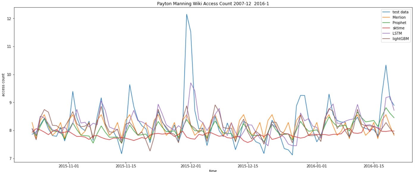
R2スコア、RMSEで5つの学習モデルの精度を比較してみましょう。
Merlion
R2スコア 0.2024673792611913
RMSE 0.6990555856934613
Prophet
R2スコア 0.22214304369582694
RMSE 0.6903786500518649
sktime
R2スコア -0.33466817117596226
RMSE 0.9043241612176715
LSTM
R2スコア 0.3802514812581941
RMSE 0.6162333966476304
lightGBM
R2スコア 0.23790827835953354
RMSE 0.6833467046462421
いずれも正規化等の処理を行っていませんし、特にlightGBM については別途特徴量を作成しているため、一概には言えないですが、LSTM の精度が一番よくなりました。
また、かなり見づらいですが、5つを比較したグラフはこちら。
以上になります、最後までお読みいただきありがとうございました。
Discussion