選挙結果をSankey diagramで可視化する

きっかけと概要

Facebookで流れてきたこの投稿を見て、選挙結果の可視化ならデータがあればサクッとできそう。

https://www.facebook.com/masashi.hagihara/posts/pfbid02hsqJhJihxjQDxxdd1q2eaP8RkQRuFtCura7bWmsHSh3moQ7mujjaNWyoGBiimYT9l

と思い立ち実装してみました。

この記事では比例代表の選挙結果の取得・前処理・Sankey diagramでの可視化、までをまとめます。

成果物

可視化したグラフはこちらに置いてあります。
縦に長いため，見切れてしまう場合はブラウザをズームアウトしていただければと思います。

データの取得

まずデータの取得です。今回は令和４年７月１０日執行の参議院議員通常選挙の速報結果のページにある都道府県別比例代表の得票数のデータを利用しました。

前処理

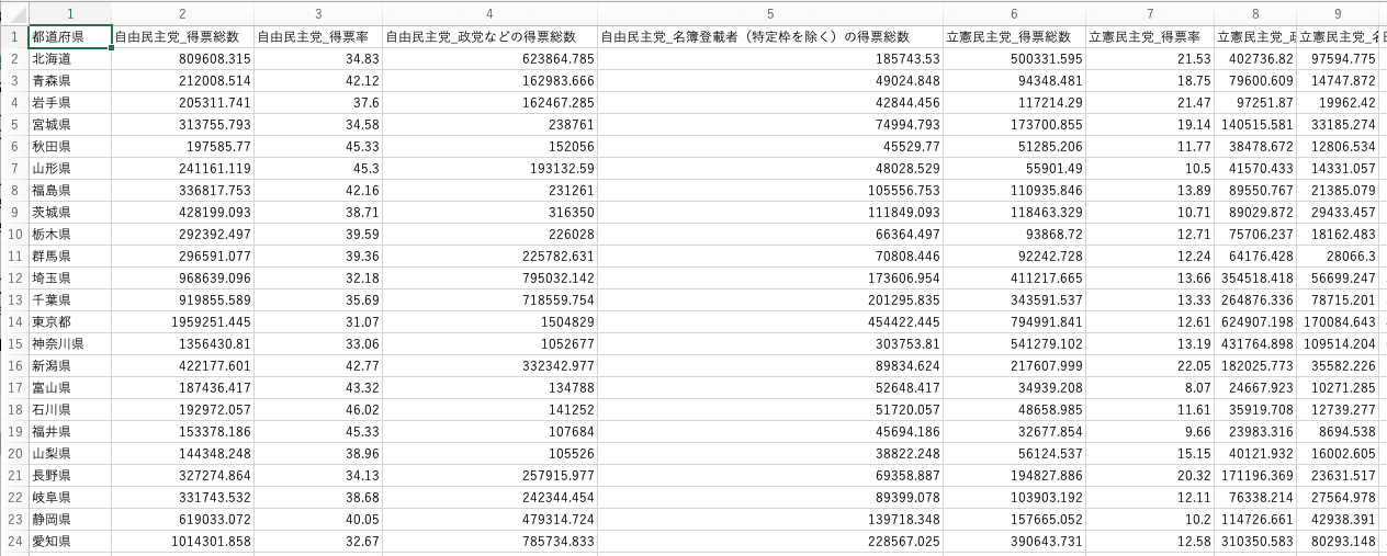
例によって神エクセルだったので、泣く泣くExcelで開き列名などを修正しました。
Excelでの作業は最低限に，残りはRで前処理を行いました。

最終的に添付の画像のようなCSVに整形しました。

plotlyで可視化

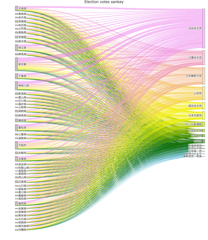
今回はRを使って可視化を行いました。野球と異なり全ての都道府県から全ての政党へのエッジがあるため、瞬発的な解釈性はあまり高くない気がします（綺麗ですが）。
しかし、じっくりと見ると各政党の基盤がどの県にあるのかが見えてきます。
また時系列的な変化も可視化できるとさらに面白いなと思いました。

そのためにも、データの形式はシンプルに一貫した形で公開してほしいと思います。

以下に参考までにコードを置いておきます。

library(plotly)
library(circlize)
library(tidyverse)

# df <- read_csv("data/processed.csv")
df <- read_csv("data/R4-7-10-election-result-processed.csv")

# 得票総数の列に絞る
preprosessor_before_sankey <- function(df){
  sankey_data <- df %>% 
    select(`都道府県`, ends_with("_得票総数"))
  
  new_colnames <- str_split(colnames(sankey_data), '_', simplify = TRUE)[,1]
  colnames(sankey_data) <- new_colnames
  colnames(sankey_data)[1] <- "都道府県"
  
  sankey_data <- sankey_data %>% 
    rename(prefecture = `都道府県`) %>% 
    pivot_longer(
      cols = c(-prefecture),
      names_to = c("party"),
      values_to = c('votes')
    )

  return(sankey_data)  
}

sankey_data <- preprosessor_before_sankey(df)
prefectures <- unique(sankey_data$prefecture)
parties     <- unique(sankey_data$party)
labels      <- c(prefectures, parties)

map_label2num <- tibble(
  label = labels,
  index = (1:length(labels)) - 1
)

# node position
step_left  <- 0.01
step_right <- 0.1
node_position <- bind_rows(
  tibble(
    label = prefectures,
    x = 0.01,
    # y = seq(0, 1, length = length(prefectures))
    y = seq(step_left, step_left*(length(prefectures)), step_left)
  ),
  tibble(
    label = parties,
    x = 0.99,
    # y = seq(0, 1, length = length(parties))
    y = seq(step_right, step_left*(length(prefectures)), length = length(parties))
  )
)

# link color: 政党の色に分ける
# Function to create colormap
create_colormap <- function(num_colors) {
  # Create breakpoints and corresponding colors
  breakpoints <- seq(0, 1, length.out = num_colors)
  colors <- colorRampPalette(c("violet","yellow", "darkgreen", "skyblue"))(num_colors)
  
  # Create a colormap
  colormap <- colorRamp2(breakpoints, colors)
  
  return(colormap)
}

# Function to convert hex color to RGBA
hex_to_rgba <- function(hex_color, alpha=1) {
  # Remove leading '#' if present
  hex_color <- gsub("^#", "", hex_color)
  
  # Extract red, green, blue components
  red_hex <- substr(hex_color, 1, 2)
  green_hex <- substr(hex_color, 3, 4)
  blue_hex <- substr(hex_color, 5, 6)
  
  # Convert to decimal
  red_dec <- as.integer(paste0("0x", red_hex))
  green_dec <- as.integer(paste0("0x", green_hex))
  blue_dec <- as.integer(paste0("0x", blue_hex))
  
  # Create RGBA string
  rgba_color <- sprintf("rgba(%d, %d, %d, %g)", red_dec, green_dec, blue_dec, alpha)
  
  return(rgba_color)
}

# Number of colors
num_colors_party <- length(parties)
num_colors_pref  <- length(prefectures)

# Create colormap
colormap_party <- create_colormap(num_colors_party)
colormap_pref  <- create_colormap(num_colors_pref)

# Map some sample values to colors
party_colors <- colormap_party(seq(0, 1, length.out = num_colors_party))
# pref_colors  <- colormap_pref(seq(0, 1, length.out = num_colors_pref))
pref_colors <- rep("#808080", num_colors_pref)
label_colors <- c(pref_colors, party_colors)

link_colors <- sankey_data %>% 
  left_join(
    tibble(
      party = parties,
      color = party_colors
    ),
    by = c("party")
  ) %>% 
  pull(color)


# Define source nodes
source <- sankey_data %>% 
  left_join(
    map_label2num, 
    by = join_by(prefecture == label)) %>% 
  pull(index)

# Define target nodes
target <- sankey_data %>% 
  left_join(
    map_label2num, 
    by = join_by(party == label)) %>% 
  pull(index)

# Define value for each link between source and target
value <- sankey_data$votes

# Create Sankey plot using plotly
fig <- plot_ly(
  type = "sankey",
  arrangement = "snap",
  
  node = list(
    pad = 10,
    thickness = 10,
    label = labels,
    x = node_position$x,
    y = node_position$y,
    color = hex_to_rgba(label_colors, alpha=0.5)
  ),
  
  link = list(
    source = source,
    target = target,
    value  = value,
    color  = hex_to_rgba(link_colors, alpha=0.5),
    label  = value
  )
) %>% plotly::layout(
  title = "Election votes sankey",
  font = list(
    size = 11
  ),
  autosize = F,
  height = 1000
)

# Show the plot
fig