Closed1ヶ月前にクローズ6

VLMを使った多言語ドキュメントパーサ「dots.ocr」を試す

OCR

VLM

dotsocr

kun432

https://huggingface.co/rednote-hilab/dots.ocr
GPT-5による翻訳

 dots.ocrdots.ocr: 単一のビジョン・ランゲージモデルによる多言語ドキュメントレイアウト解析

 はじめにdots.ocr は強力な多言語ドキュメントパーサであり、単一のビジョン・ランゲージモデル内でレイアウト検出とコンテンツ認識を統合し、良好な読順を維持します。1.7BパラメータのLLM基盤というコンパクトさにもかかわらず、最先端（SOTA）の性能を達成しています。

強力な性能: dots.ocr は OmniDocBench において、テキスト・表・読順でSOTA性能を達成し、数式認識においても Doubao-1.5 や gemini2.5-pro のようなより大規模なモデルに匹敵する結果を示します。

多言語対応: dots.ocr はリソースの少ない言語に対しても堅牢な解析能力を示し、自社の多言語ドキュメントベンチマークにおいて、レイアウト検出とコンテンツ認識の両面で明確な優位性を獲得しています。

統合されたシンプルなアーキテクチャ: 単一のビジョン・ランゲージモデルを活用することで、従来の複雑なマルチモデルパイプラインに比べて大幅に効率的なアーキテクチャを実現しています。タスクの切り替えは入力プロンプトを変更するだけで行え、DocLayout-YOLO のような従来型の検出モデルに匹敵する競争力を示します。

効率的かつ高速: コンパクトな1.7B LLMに基づくため、より大規模な基盤に依存する多くの高性能モデルに比べて推論速度が速くなっています。

 性能比較: dots.ocr vs. 競合モデル

referred from https://huggingface.co/rednote-hilab/dots.ocr
注記:
EN、ZHの指標は OmniDocBench によるend-to-end評価結果。
Multilingual の指標は dots.ocr-bench によるend-to-end評価結果。
その他ベンチマークや実際のドキュメント読み取り結果などはモデルカード参照
ライセンスはMITライセンス。

kun432

GitHubレポジトリ
https://github.com/rednote-hilab/dots.ocr?tab=readme-ov-file
ブログ、というかGitHubレポジトリにあるドキュメント。書いてあることは概ねモデルカードと同じように思うが、学習過程について少し記述がある
https://github.com/rednote-hilab/dots.ocr/tree/master/assets/blog.md
以下でデモが試せる。
https://dotsocr.xiaohongshu.com/

kun432

まずはColaboratory L4で。

レポジトリクローン

!git clone https://github.com/rednote-hilab/dots.ocr.git
%cd dots.ocr

パッケージインストール。Colaboratory環境に合わせて少し変えている。

!pip install torch==2.4.0 torchvision==0.19.0 torchaudio==2.4.0 --index-url https://download.pytorch.org/whl/cu124
!pip install -e .

モデルをダウンロード

!python3 tools/download_model.py

推論は、vLLM / HuggingFace （というかtransformers）など、それぞれにあわせたPythonスクリプトをCLIで実行する形で提供されているが、ここではtransformersのコードを使うことにする。

モデルとプロセッサをロード

import torch
from transformers import AutoModelForCausalLM, AutoProcessor, AutoTokenizer
from qwen_vl_utils import process_vision_info
from dots_ocr.utils import dict_promptmode_to_prompt

model_path = "./weights/DotsOCR"
model = AutoModelForCausalLM.from_pretrained(
    model_path,
    attn_implementation="flash_attention_2",
    torch_dtype=torch.bfloat16,
    device_map="auto",
    trust_remote_code=True
)
processor = AutoProcessor.from_pretrained(model_path, trust_remote_code=True)

この時点でのVRAM消費は6GB。

出力

+-----------------------------------------------------------------------------------------+
| NVIDIA-SMI 550.54.15              Driver Version: 550.54.15      CUDA Version: 12.4     |
|-----------------------------------------+------------------------+----------------------+
| GPU  Name                 Persistence-M | Bus-Id          Disp.A | Volatile Uncorr. ECC |
| Fan  Temp   Perf          Pwr:Usage/Cap |           Memory-Usage | GPU-Util  Compute M. |
|                                         |                        |               MIG M. |
|=========================================+========================+======================|
|   0  NVIDIA L4                      Off |   00000000:00:03.0 Off |                    0 |
| N/A   41C    P0             27W /   72W |    6043MiB /  23034MiB |      0%      Default |
|                                         |                        |                  N/A |
+-----------------------------------------+------------------------+----------------------+

では推論。レポジトリの中にサンプルの画像が含まれていて、これを推論するものとなっている。

from IPython.display import Image

image_path = "demo/demo_image1.jpg"
display(Image(image_path, width=1024))

元の画像ファイルはここ。何かしらの論文の表部分みたい。

では推論。

image_path = "demo/demo_image1.jpg"
prompt = """Please output the layout information from the PDF image, including each layout element's bbox, its category, and the corresponding text content within the bbox.

1. Bbox format: [x1, y1, x2, y2]

2. Layout Categories: The possible categories are ['Caption', 'Footnote', 'Formula', 'List-item', 'Page-footer', 'Page-header', 'Picture', 'Section-header', 'Table', 'Text', 'Title'].

3. Text Extraction & Formatting Rules:
    - Picture: For the 'Picture' category, the text field should be omitted.
    - Formula: Format its text as LaTeX.
    - Table: Format its text as HTML.
    - All Others (Text, Title, etc.): Format their text as Markdown.

4. Constraints:
    - The output text must be the original text from the image, with no translation.
    - All layout elements must be sorted according to human reading order.

5. Final Output: The entire output must be a single JSON object.
"""

messages = [
        {
            "role": "user",
            "content": [
                {
                    "type": "image",
                    "image": image_path
                },
                {"type": "text", "text": prompt}
            ]
        }
    ]

# Preparation for inference
text = processor.apply_chat_template(
    messages, 
    tokenize=False, 
    add_generation_prompt=True
)
image_inputs, video_inputs = process_vision_info(messages)
inputs = processor(
    text=[text],
    images=image_inputs,
    videos=video_inputs,
    padding=True,
    return_tensors="pt",
)

inputs = inputs.to("cuda")

# Inference: Generation of the output
generated_ids = model.generate(**inputs, max_new_tokens=24000)
generated_ids_trimmed = [
    out_ids[len(in_ids) :] for in_ids, out_ids in zip(inputs.input_ids, generated_ids)
]
output_text = processor.batch_decode(
    generated_ids_trimmed, skip_special_tokens=True, clean_up_tokenization_spaces=False
)
print(output_text)

3分ほどで結果が返ってきた。ちょっと結果が長くて見にくいので少し分解。

import json

for i in json.loads(output_text[0]):
    print(i)

出力

{'bbox': [628, 172, 1077, 193], 'category': 'Page-header', 'text': 'EXPOSURE TO MEAT AND RISK OF LYMPHOMA'}
{'bbox': [1487, 169, 1540, 193], 'category': 'Page-header', 'text': '2763'}
{'bbox': [278, 217, 1428, 237], 'category': 'Caption', 'text': 'TABLE II - ODDS RATIO OF HODGKIN LYMPHOMA AND NON-HODGKIN LYMPHOMA FOR INDICATORS OF EXPOSURE TO MEAT'}
{'bbox': [164, 240, 1540, 700], 'category': 'Table', 'text': '<table><thead><tr><th rowspan="2"></th><th rowspan="2">Controls</th><th colspan="3">Hodgkin lymphoma</th><th colspan="3">Non-Hodgkin lymphoma</th></tr><tr><th>Cases</th><th>OR</th><th>95% CI</th><th>Cases</th><th>OR</th><th>95% CI</th></tr></thead><tbody><tr><td>Never Exposed (reference group)</td><td>2,273</td><td>315</td><td>1.00</td><td>—</td><td>1,823</td><td>1.00</td><td>—</td></tr><tr><td>Ever Exposed</td><td>189</td><td>24</td><td>1.06</td><td>0.65–1.71</td><td>184</td><td>1.18</td><td>0.95–1.46</td></tr><tr><td>Duration of exposure</td><td></td><td></td><td></td><td></td><td></td><td></td><td></td></tr><tr><td>≤5 years</td><td>52</td><td>12</td><td>1.14</td><td>0.57–2.30</td><td>49</td><td>1.25</td><td>0.84–1.86</td></tr><tr><td>6–15 years</td><td>62</td><td>8</td><td>0.98</td><td>0.44–2.20</td><td>52</td><td>1.04</td><td>0.71–1.51</td></tr><tr><td>≥16 years</td><td>73</td><td>4</td><td>1.02</td><td>0.36–2.90</td><td>82</td><td>1.27</td><td>0.92–1.76</td></tr><tr><td>p-value of test for linear trend</td><td></td><td></td><td></td><td>0.90</td><td></td><td></td><td>0.13</td></tr><tr><td>Weighted duration of exposure</td><td></td><td></td><td></td><td></td><td></td><td></td><td></td></tr><tr><td>≤6 months</td><td>62</td><td>14</td><td>1.54</td><td>0.79–2.99</td><td>57</td><td>1.10</td><td>0.76–1.59</td></tr><tr><td>7 months to 1 year</td><td>35</td><td>3</td><td>0.60</td><td>0.17–2.13</td><td>40</td><td>1.39</td><td>0.87–2.20</td></tr><tr><td>>1 year</td><td>90</td><td>7</td><td>0.84</td><td>0.37–1.91</td><td>86</td><td>1.17</td><td>0.87–1.59</td></tr><tr><td>p-value of test for linear trend</td><td></td><td></td><td></td><td>0.75</td><td></td><td></td><td>0.13</td></tr><tr><td>Intensity of exposure</td><td></td><td></td><td></td><td></td><td></td><td></td><td></td></tr><tr><td>Low</td><td>84</td><td>11</td><td>1.05</td><td>0.52–2.12</td><td>85</td><td>1.24</td><td>0.91–1.70</td></tr><tr><td>Medium</td><td>70</td><td>10</td><td>1.19</td><td>0.56–2.49</td><td>66</td><td>1.11</td><td>0.79–1.57</td></tr><tr><td>High</td><td>35</td><td>3</td><td>0.80</td><td>0.23–2.74</td><td>32</td><td>1.14</td><td>0.70–1.85</td></tr></tbody></table>'}
{'bbox': [188, 715, 1213, 741], 'category': 'Text', 'text': 'OR, odds ratio, adjusted for age, sex, center, and cumulative exposure to pesticides; CI, confidence interval.'}
{'bbox': [315, 824, 1390, 844], 'category': 'Caption', 'text': 'TABLE III - ODDS RATIO OF ALL NON-HODGKIN LYMPHOMA FOR EXPOSURE TO SPECIFIC TYPES OF MEAT-ALL NHL'}
{'bbox': [164, 846, 1540, 1266], 'category': 'Table', 'text': '<table><thead><tr><th rowspan="2"></th><th colspan="4">Beef meat</th><th colspan="4">Chicken meat</th><th colspan="4">Pork meat</th></tr><tr><th>Cases</th><th>Controls</th><th>OR</th><th>95% CI</th><th>Cases</th><th>Controls</th><th>OR</th><th>95% CI</th><th>Cases</th><th>Controls</th><th>OR</th><th>95% CI</th></tr></thead><tbody><tr><td>Never Exposed (Ref group)</td><td>1,823</td><td>2,273</td><td>1.00</td><td></td><td>1,823</td><td>2,273</td><td>1.00</td><td></td><td>1,823</td><td>2,273</td><td>1.00</td><td></td></tr><tr><td>Ever Exposed</td><td>117</td><td>108</td><td>1.22</td><td>0.90–1.67</td><td>1,36</td><td>129</td><td>1.19</td><td>0.91–1.55</td><td>145</td><td>143</td><td>1.09</td><td>0.83–1.42</td></tr><tr><td>Duration of exposure</td><td></td><td></td><td></td><td></td><td></td><td></td><td></td><td></td><td></td><td></td><td></td><td></td></tr><tr><td>≤5 years</td><td>40</td><td>37</td><td>1.45</td><td>0.92–2.31</td><td>30</td><td>40</td><td>0.97</td><td>0.60–1.58</td><td>39</td><td>41</td><td>1.25</td><td>0.80–1.96</td></tr><tr><td>6–15 years</td><td>29</td><td>43</td><td>0.79</td><td>0.47–1.31</td><td>42</td><td>41</td><td>1.21</td><td>0.78–1.88</td><td>44</td><td>58</td><td>0.84</td><td>0.55–1.28</td></tr><tr><td>≥16 years</td><td>48</td><td>28</td><td>1.63</td><td>0.93–2.88</td><td>64</td><td>48</td><td>1.36</td><td>0.90–2.06</td><td>61</td><td>43</td><td>1.28</td><td>0.81–2.03</td></tr><tr><td>p-value of test for linear trend (with ref cat)</td><td></td><td></td><td>0.23</td><td></td><td></td><td></td><td>0.11</td><td></td><td></td><td></td><td>0.54</td><td></td></tr><tr><td>Intensity of exposure</td><td></td><td></td><td></td><td></td><td></td><td></td><td></td><td></td><td></td><td></td><td></td><td></td></tr><tr><td>Low</td><td>60</td><td>59</td><td>1.26</td><td>0.86–1.83</td><td>71</td><td>68</td><td>1.24</td><td>0.88–1.75</td><td>70</td><td>72</td><td>1.15</td><td>0.82–1.62</td></tr><tr><td>Medium</td><td>42</td><td>35</td><td>1.22</td><td>0.73–2.04</td><td>47</td><td>46</td><td>1.11</td><td>0.72–1.71</td><td>55</td><td>52</td><td>1.03</td><td>0.68–1.58</td></tr><tr><td>High</td><td>15</td><td>14</td><td>0.91</td><td>0.35–2.40</td><td>18</td><td>15</td><td>1.22</td><td>0.56–2.65</td><td>20</td><td>19</td><td>0.89</td><td>0.40–1.94</td></tr><tr><td>p-value of test for linear trend (with ref cat)</td><td></td><td></td><td>0.36</td><td></td><td></td><td></td><td>0.29</td><td></td><td></td><td></td><td>0.78</td><td></td></tr></tbody></table>'}
{'bbox': [164, 1268, 1540, 1683], 'category': 'Table', 'text': '<table><thead><tr><th rowspan="2"></th><th colspan="4">Mutton meat</th><th colspan="4">Other meat</th></tr><tr><th>Cases</th><th>Controls</th><th>OR</th><th>95% CI</th><th>Cases</th><th>Controls</th><th>OR</th><th>95% CI</th></tr></thead><tbody><tr><td>Never Exposed (Ref group)</td><td>1,823</td><td>2,273</td><td>1.00</td><td></td><td>1,823</td><td>2,273</td><td>1.00</td><td></td></tr><tr><td>Ever Exposed</td><td>63</td><td>71</td><td>0.99</td><td>0.66–1.47</td><td>52</td><td>47</td><td>1.07</td><td>0.67–1.70</td></tr><tr><td>Duration of exposure</td><td></td><td></td><td></td><td></td><td></td><td></td><td></td><td></td></tr><tr><td>≤5 years</td><td>21</td><td>20</td><td>1.35</td><td>0.71–2.56</td><td>13</td><td>15</td><td>0.92</td><td>0.41–2.06</td></tr><tr><td>6–15 years</td><td>21</td><td>27</td><td>0.87</td><td>0.46–1.62</td><td>13</td><td>10</td><td>1.16</td><td>0.48–2.81</td></tr><tr><td>≥16 years</td><td>21</td><td>24</td><td>0.80</td><td>0.41–1.57</td><td>26</td><td>21</td><td>1.19</td><td>0.62–2.28</td></tr><tr><td>p-value of test for linear trend (with ref cat)</td><td></td><td></td><td>0.60</td><td></td><td></td><td></td><td>0.58</td><td></td></tr><tr><td>Intensity of exposure</td><td></td><td></td><td></td><td></td><td></td><td></td><td></td><td></td></tr><tr><td>Low</td><td>31</td><td>41</td><td>0.90</td><td>0.55–1.47</td><td>24</td><td>30</td><td>0.82</td><td>0.47–1.45</td></tr><tr><td>Medium</td><td>22</td><td>21</td><td>1.11</td><td>0.57–2.14</td><td>17</td><td>8</td><td>1.97</td><td>0.80–4.90</td></tr><tr><td>High</td><td>10</td><td>9</td><td>1.29</td><td>0.42–4.00</td><td>10</td><td>9</td><td>1.09</td><td>0.34–3.51</td></tr><tr><td>p-value of test for linear trend (with ref cat)</td><td></td><td></td><td>0.80</td><td></td><td></td><td></td><td>0.57</td><td></td></tr></tbody></table>'}
{'bbox': [188, 1698, 1395, 1724], 'category': 'Text', 'text': 'OR, odds ratio adjusted for age, sex, center, cumulative exposure to pesticides and other types of meat; CI, confidence interval.'}
{'bbox': [164, 1774, 839, 1854], 'category': 'Text', 'text': 'sponding OR of non-Hodgkin lymphoma was 1.18 (95% CI 0.95–1.46): also for this group of lymphoma, no trend was apparent for any indicator of exposure.'}
{'bbox': [164, 1858, 839, 2068], 'category': 'Text', 'text': 'When the analysis on non-Hodgkin lymphoma was repeated for specific types of meat (Table III), the OR for ever exposure to beef meat was 1.22 (95% CI 0.95–1.67), and the OR for ever exposure to chicken meat was 1.19 (95% CI 0.91–1.55). The remaining meat types, namely pork meat and mutton meat, showed either no effect or small nonsignificant increases in lymphoma risk. Exposure for more than 15 years to beef meat resulted in an OR of 1.63 (95% CI 0.93–2.88). An increase in risk was also observed'}
{'bbox': [867, 1774, 1540, 1854], 'category': 'Text', 'text': 'for long-term exposure to chicken meat (OR = 1.36, 95% CI 0.90–2.06). The results on intensity of exposure did not suggest a difference among meat types.'}
{'bbox': [867, 1858, 1540, 2068], 'category': 'Text', 'text': 'In the analyses stratified by lymphoma type, whose results are reported in Table IV, an increased risk among workers exposed to beef meat was mainly apparent for diffuse large B-cell lymphoma (OR = 1.49, 95% CI 0.96–2.33), chronic lymphocytic leukemia/small lymphocytic lymphoma (OR = 1.35, 95% CI 0.78–2.34), and multiple myeloma (OR = 1.40, 95% CI 0.67–2.94). Stronger increases in risk were observed for each of these 3 subtypes after 16 years or more of exposure (OR 2.00, 95% CI 0.87–4.61; OR'}

文字を認識した箇所をバウンディングボックスで抽出して、文書レイアウト上におけるカテゴリ名、そして認識した文字を抽出しているのがわかる。

なお、推論で使用されていたプロンプトの日本語訳はこんな感じ。

PDF画像からレイアウト情報を出力してください。各レイアウト要素のバウンディングボックス（bbox）、そのカテゴリ、およびbbox内の対応するテキストコンテンツを含めます。

Bbox 形式: [x1, y1, x2, y2]

レイアウトカテゴリ: 可能なカテゴリは ['Caption', 'Footnote', 'Formula', 'List-item', 'Page-footer', 'Page-header', 'Picture', 'Section-header', 'Table', 'Text', 'Title'] です。

テキスト抽出とフォーマット規則:

画像: 『画像』カテゴリの場合、テキストフィールドは省略します。

数式: テキストをLaTeX形式でフォーマットします。

表: テキストをHTML形式でフォーマットします。

その他のすべて（テキスト、タイトルなど）：テキストをMarkdown形式でフォーマットします。

制約：

出力テキストは画像元のテキストそのもので、翻訳は行わないこと。

すべてのレイアウト要素は人間の読み順に従って並べ替えること。

最終出力：出力全体は単一のJSONオブジェクトでなければならない。

kun432

全体的にCLIでの利用が想定されているように見受けられるので、ここからはローカルでやる。Ubuntu-22.04 + RTX4090 + CUDA-12.8 環境で。

レポジトリクローン

git clone https://github.com/rednote-hilab/dots.ocr && cd dots.ocr

Python仮想環境を作成（今回はuvはこのためだけ）。

uv venv -p 3.12
uv pip install pip
source .venv/bin/activate

パッケージインストール

pip install torch==2.7.0 torchvision==0.22.0 torchaudio==2.7.0 --index-url https://download.pytorch.org/whl/cu128
pip install -e .

が、pip install -e . で flash-attnをインストールするようになっているのだが、これのビルドでどうもコケる。

出力

Collecting flash-attn==2.8.0.post2 (from dots_ocr==1.0)
  Using cached flash_attn-2.8.0.post2.tar.gz (7.9 MB)
  Installing build dependencies ... done
  Getting requirements to build wheel ... error
  error: subprocess-exited-with-error

  × Getting requirements to build wheel did not run successfully.
  │ exit code: 1
  ╰─> [20 lines of output]
(snip)
        File "<string>", line 22, in <module>
      ModuleNotFoundError: No module named 'torch'
      [end of output]

  note: This error originates from a subprocess, and is likely not a problem with pip.
error: subprocess-exited-with-error

× Getting requirements to build wheel did not run successfully.
│ exit code: 1
╰─> See above for output.

note: This error originates from a subprocess, and is likely not a problem with pip.

以下で回避できた。

pip install -U setuptools wheel

モデルダウンロード

python tools/download_model.py

モデルを動かすAPIサーバをvLLMで起動する。というかvLLMのインストールについてはどこにも書かれていなくて、諸々わかりにくい・・・

pip install vllm

export hf_model_path=./weights/DotsOCR
export PYTHONPATH=$(dirname "$hf_model_path"):$PYTHONPATH
sed -i '/^from vllm\.entrypoints\.cli\.main import main$/a\
from DotsOCR import modeling_dots_ocr_vllm' `which vllm`

CUDA_VISIBLE_DEVICES=0 vllm serve ${hf_model_path} --tensor-parallel-size 1 --gpu-memory-utilization 0.95  --chat-template-content-format string --served-model-name model --trust-remote-code

こんな感じで表示されればOK。

出力

(snip)
INFO 08-18 22:17:51 [api_server.py:1818] Starting vLLM API server 0 on http://0.0.0.0:8000
(snip)
INFO:     Started server process [3474729]
INFO:     Waiting for application startup.
INFO:     Application startup complete.

次に別ターミナルを開いて、今度はGradioのデモを起動する。最後の引数はポート番号を指定。

python demo/demo_gradio.py 7860

ブラウザでアクセスすると、公式のデモと同じ画面が開く。

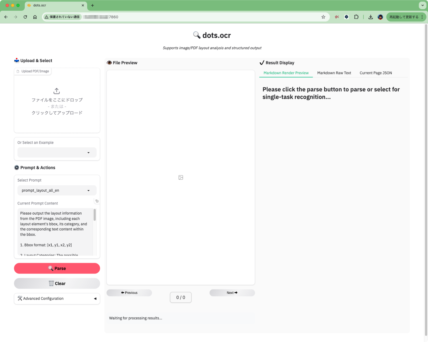
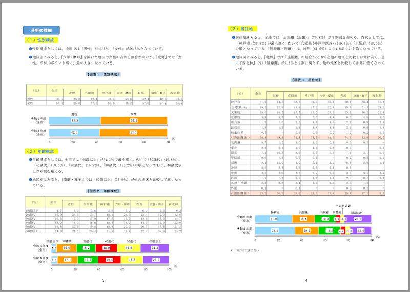
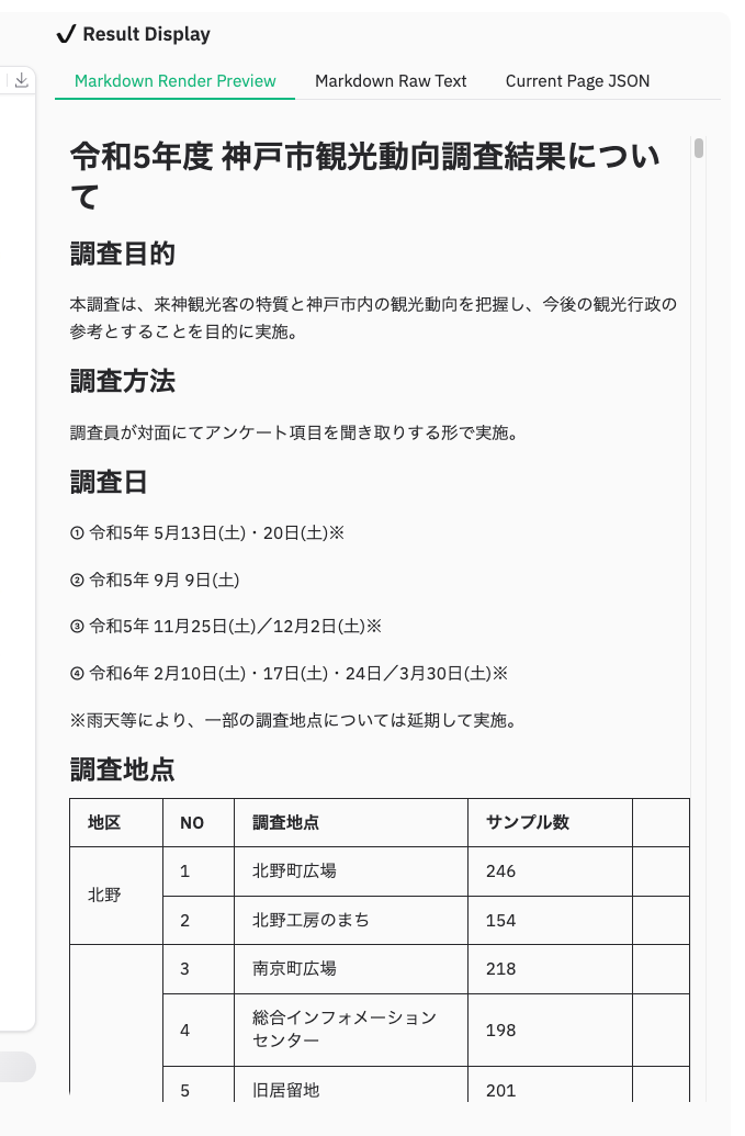
ではPDFをアップロードしてみる。サンプルとして、神戸市が公開している観光に関する統計・調査資料のうち、「令和5年度神戸市観光動向調査結果について」のPDFを使用させていただく。

PDFの特徴

サイズ: 1.8MB
ページ数: 21
縦長レイアウト
文字は横書き
表・グラフ等含む

参考までに一部抜粋。

では、PDFをアップロード

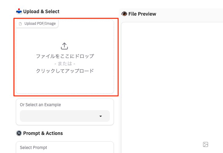
アップロードされたら、"Parse"をクリック。プロンプトなども変更できるようだが、一旦このままで。

今回は21ページのPDFなので、順に解析が行われる。Gradioデモを開いたコンソールにはこんな感じで進捗が表示されている。

出力

Parsing PDF with 21 pages using 21 threads...
Processing PDF pages:  76%|███████████████████████████████████████████████▏              | 16/21 [00:49<00:02,  1.68it/s]

パースできた様子。こんな感じで表示される。

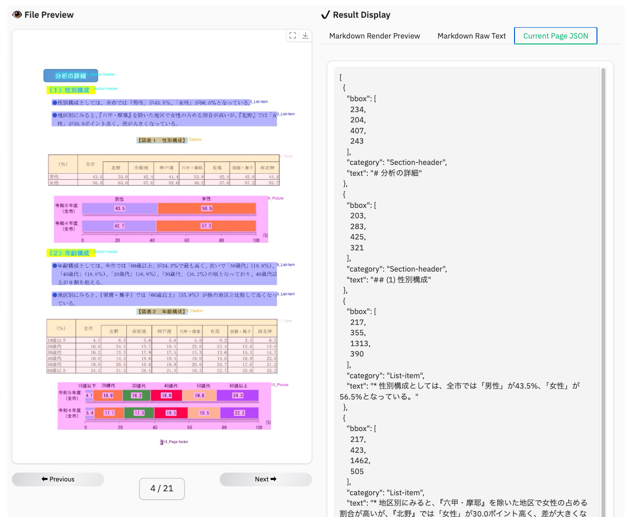
各ページはこんな感じでレイアウトパーツごとに解析されているのがわかる。

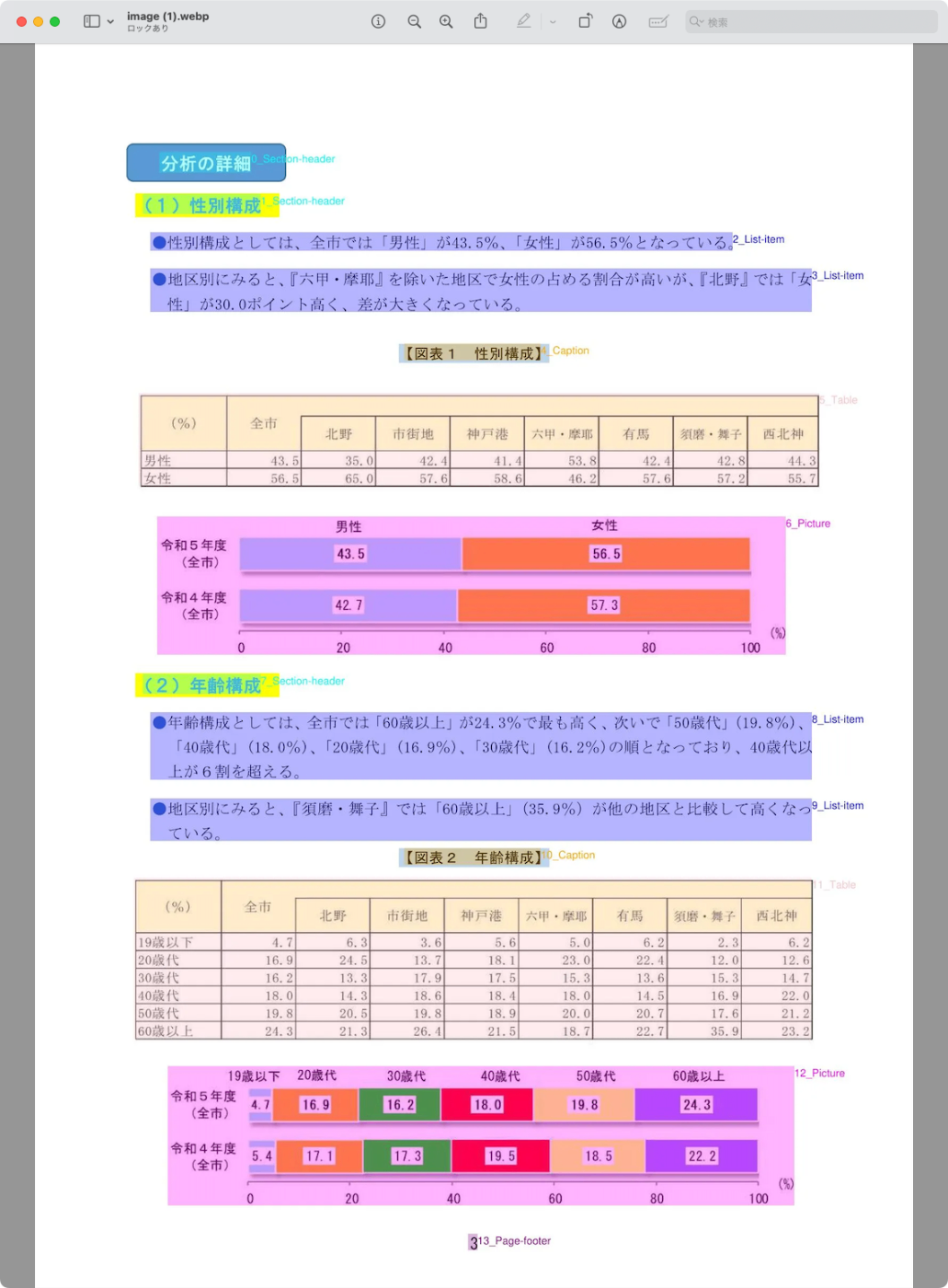
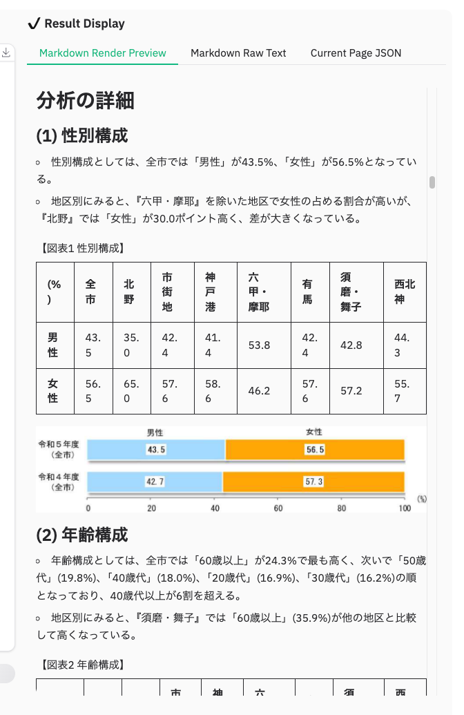
解析結果は、レンダリングされたMarkdownでの表示と生のMarkdown出力が行われる。グラフなどの画像部分は画像として抽出されてレンダリングされていた。

上記は全ページ分まとめてになるが、現在見ているページごとに解析結果をJSONで見ることもできる。

結果はzipでまとめてダウンロードできる。

ダウンロードしたZIPの中身はこんな感じ。

出力

layout_results_48294ba4
├── demo_48294ba4_page_0.jpg
├── demo_48294ba4_page_0.json
├── demo_48294ba4_page_0.md
├── demo_48294ba4_page_0_nohf.md
├── demo_48294ba4_page_1.jpg
├── demo_48294ba4_page_1.json
├── demo_48294ba4_page_1.md
├── demo_48294ba4_page_10.jpg
├── demo_48294ba4_page_10.json
├── demo_48294ba4_page_10.md
├── demo_48294ba4_page_10_nohf.md
├── demo_48294ba4_page_11.jpg
├── demo_48294ba4_page_11.json
├── demo_48294ba4_page_11.md
├── demo_48294ba4_page_11_nohf.md
├── demo_48294ba4_page_12.jpg
├── demo_48294ba4_page_12.json
├── demo_48294ba4_page_12.md
├── demo_48294ba4_page_12_nohf.md
(snip)

各ページごとに

*.jpg: ページのレイアウト解析後の画像
*.json: ページのレイアウト解析及びOCR後のJSON
*.md: ページを解析・OCR後のMarkdown
*_nohf.md: ページを解析・OCR後のMarkdown。おそらくだが、ページのヘッダー・フッターなしバージョン。

という感じで出力される。なお、文書中の画像はBASE64文字列としてMarkdownに埋め込まれていた。

あと上記以外に、

画像からアノテーションを行うGradioデモ
PDFや画像の解析を行うCLI

などもある。

kun432

精度や実行速度などについて。

個人的な印象ではあるが、概ねいい感じの精度で解析できているのではないかと思う。ただ複雑な表の場合には上手く抽出できていないケースもあった。
上記の21ページのPDFで1分ほどだった。1ページあたり3秒程度となるが、おそらくPDFの初期処理を行う箇所では多少時間がかかっていたように思う。

kun432

 まとめ多少手順が不親切なところはあるが、Gradioのデモが起動できたら、あとはとても使いやすいと思うし、精度も結構良いのではないかと思う。大量に処理するようなケースであればCLIも使えるのも良い。
今回は試してないけど、解析時にはプロンプトを指定できるんだよね。ここの指定の仕方で、解析精度が向上するとか、ほしい出力に調整するとか、できるんだろうか？そういうのもできるとより便利に使えるかもしれない。

このスクラップは1ヶ月前にクローズされました