Librosaで扱える音響特徴量まとめ

はじめに

本記事では、Librosa 0.10.1で利用することが出来る音響特徴量を紹介します。
あくまでもライブラリの紹介なので、それぞれの関数の概要を紹介し、詳細については深追いしません。

Librosaとは

Librosaは、Pythonの音響解析および信号処理のライブラリです。
音響特徴量の抽出から、テンポ・ビート推定、和音推定、オーディオ編集、エフェクト処理、周波数への変換など、オーディオ処理なら何でも出来ちゃうライブラリです。

Chromagram

クロマグラムです。周波数から12音階のパワーを算出し、時間軸ごとにどの音階が鳴っているかを表す2次元配列として出力されます。和音推定などに応用されます。

Librosaでは4種類(STFT, CQT, CENS, VQT)のクロマグラム関数があり、それぞれ算出のアルゴリズムが異なるので、適した関数を選択する必要があります。今回は最も一般的であろうSTFTでのクロマグラム算出を行います。

import librosa
import librosa.display
import matplotlib.pyplot as plt

y, sr = librosa.load('demo.mp3')
chromagram = librosa.feature.chroma_stft(y=y, sr=sr)

plt.figure(figsize=(12, 4))
librosa.display.specshow(chromagram, y_axis='chroma', x_axis='time')
plt.colorbar()
plt.title('Chromagram')
plt.tight_layout()
plt.show()

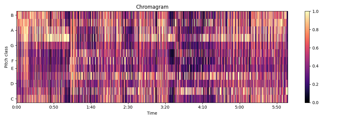
ある曲のクロマグラムを算出した結果です。D♭,E♭,A♭,B♭あたりが若干強めだなと分かります。実際にこの曲のキーはE♭-minorであり、これらは全てキーの構成音なので、推定結果としては正しいと言えます。

Melspectrogram

メルスペクトログラムは、周波数軸をメル尺度にしたスペクトログラムです。メル尺度とは、人間の耳の周波数に対する感覚に基づいた音響尺度のことです。例えば、人間は500Hzの音と600Hzの音の違いは判断出来ますが、20kHzと20.1kHzの音の違いは判断が難しいといった感じです。詳しい内容については省略します。

メルスペクトログラムは、主に後述するMFCCを算出するための前処理として利用されます。

import librosa
import librosa.display
import matplotlib.pyplot as plt
import numpy as np

y, sr = librosa.load('demo.mp3')
mel_spectrogram = librosa.feature.melspectrogram(y=y, sr=sr)
mel_spectrogram_dB = librosa.power_to_db(mel_spectrogram, ref=np.max) # デシベル単位に変換

plt.figure(figsize=(12, 4))
librosa.display.specshow(mel_spectrogram_dB, x_axis='time', y_axis='mel', sr=sr)
plt.colorbar(format='%+2.0f dB')
plt.title('Mel spectrogram')
plt.tight_layout()
plt.show()

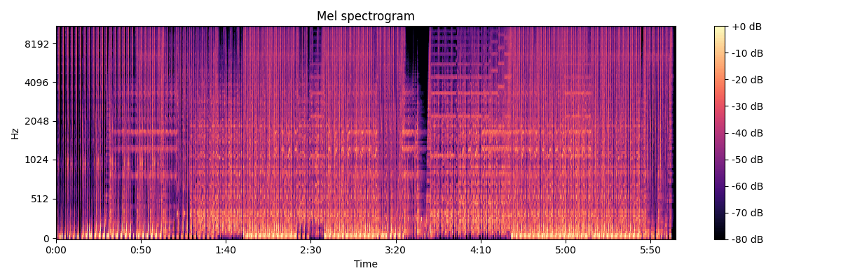
若干無理があるかもしれませんが、大体の曲の全体像をここから読み取ることが出来ます。まあこれだったら単なるスペクトログラムでいいかもしれません。

MFCC

MFCCは、人間の音の知覚に基づいたスペクトルの概形です。メルスペクトログラムをあれこれして算出することが出来ます。細かい実装方法については省略します。

NNの学習データとしてや、クラスタリングデータとして、自動音声認識、感情認識など、多くの活用事例があります。

import librosa
import librosa.display
import matplotlib.pyplot as plt

y, sr = librosa.load("demo.mp3")
mfccs = librosa.feature.mfcc(y=y, sr=sr, n_mfcc=20)

plt.figure(figsize=(12, 4))
librosa.display.specshow(mfccs, x_axis='time', sr=sr)
plt.colorbar(label='MFCC coefficient')
plt.title('MFCC')
plt.tight_layout()
plt.show()

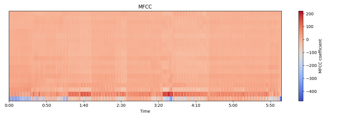
LibrosaのMFCCを使えば、メルスペクトログラムを求める過程をすっ飛ばして一発でMFCCを求めてくれます。
引数のn_mfccでは、MFCCの次元数を指定します。標準値でも20なので、大体その程度が一般的な次元数だと思われます。

曲全体をぶち込んだら、低次元の要素が強すぎてよく分かりませんでした。この記事は上手な活用法を紹介するものではないので、これで良しとします。

RMS

RMSは音圧とも呼ばれていますが、Root Means Square(二乗平均平方根)であり、音圧というより音の平均値と呼ぶ方が正確だと思います。音の持続的な強さを表す値です。例えば、ドラム音のような瞬間的な値は、持続性が無いので、RMSを算出すると値は低くなります。

import librosa
import librosa.display
import matplotlib.pyplot as plt
import numpy as np

y, sr = librosa.load("demo.mp3")
rms = librosa.feature.rms(y=y, frame_length=65000, hop_length=16250)[0]
rms /= np.max(rms) # 正規化
times = np.floor(librosa.times_like(rms, hop_length=16250, sr=44100))

plt.figure(figsize=(12, 4))
plt.plot(rms)
plt.ylabel("RMS")
plt.xlabel("time")
plt.legend()
plt.tight_layout()
plt.show()

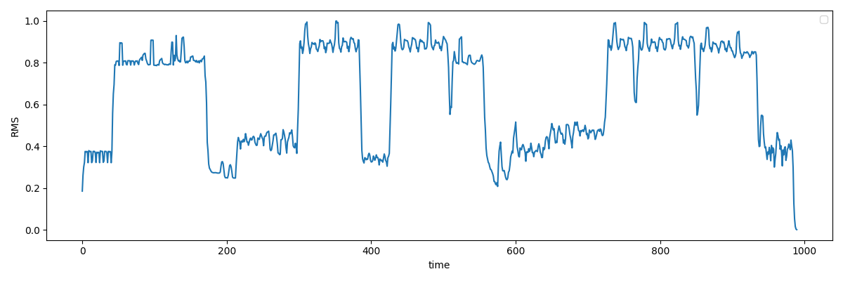
音楽においては、一般的にRMSは曲の盛り上がり具合と相関があるので、曲のどの部分が盛り上がっているかをRMSからある程度判断することが出来ます。上の図では、序盤・中盤・終盤と大きく3つの盛り上がる局面があることがわかります。

Spectral Centroid

Spectral Centroidは、その周波数を分岐点に、上下でエネルギーが釣り合う点を表す特徴量です。つまり、時間軸におけるスペクトルの中心です。スペクトル重心が低いほど周波数が低く、高いほど周波数も高いことを表します。

import librosa
import librosa.display
import matplotlib.pyplot as plt
import numpy as np

y, sr = librosa.load("demo.mp3")
spectral_centroid = librosa.feature.spectral_centroid(y=y, sr=sr)[0]
spectral_centroid = np.convolve(spectral_centroid, np.ones(200)/200, mode='valid')
times = librosa.frames_to_time(np.arange(len(spectral_centroid)), sr=sr)

plt.figure(figsize=(12, 4))
plt.plot(times, spectral_centroid)
plt.ylabel('Hz')
plt.xlabel('Time')
plt.title('Spectral Centroid')
plt.grid(True)
plt.legend()
plt.tight_layout()
plt.show()

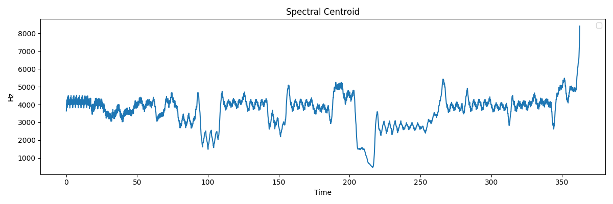
上の図の様に、曲におけるスペクトルの重心の変化が見て取れます。例えば下の図の曲だと、中盤ごろに急激にスペクトル重心が下がっている部分が特徴的です。

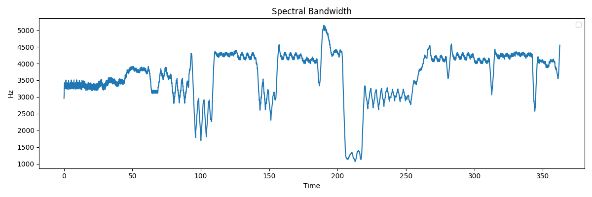
Spectral Bandwidth

Spectral Bandwidthは、スペクトルの帯域幅、つまり、その時間軸におけるスペクトルの分布の広がりを表します。値が大きいほど幅広い周波数成分を含んでおり、値が小さいほど限られた周波数成分しか含まないことを意味します。

import librosa
import librosa.display
import matplotlib.pyplot as plt
import numpy as np

y, sr = librosa.load("demo.mp3")
spectral_bandwidth = librosa.feature.spectral_bandwidth(y=y, sr=sr)[0]
spectral_bandwidth = np.convolve(spectral_bandwidth, np.ones(200)/200, mode='valid')
times = librosa.frames_to_time(np.arange(len(spectral_bandwidth)), sr=sr)

plt.figure(figsize=(12, 4))
plt.plot(times, spectral_bandwidth)
plt.ylabel('Hz')
plt.xlabel('Time (seconds)')
plt.title('Spectral Bandwidth')
plt.legend()
plt.tight_layout()
plt.show()

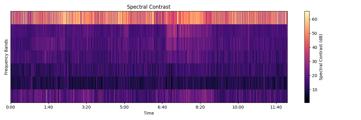
Spectral Contrast

スペクトルを6つのサブバンドに分け、それぞれのバンドにおけるコントラスト(音の強弱の差)を表します。

import librosa
import librosa.display
import matplotlib.pyplot as plt
import numpy as np

y, sr = librosa.load("demo.mp3")
spectral_contrast = librosa.feature.spectral_contrast(y=y, sr=sr)

plt.figure(figsize=(12, 4))
librosa.display.specshow(spectral_contrast, x_axis='time')
plt.colorbar(label='Spectral Contrast (dB)')
plt.ylabel('Frequency Bands')
plt.title('Spectral Contrast')
plt.tight_layout()
plt.show()

Spectral Flatness

その時間軸において、そのスペクトルがどれだけ平坦であるかを測定します。結果は0~1で表され、0に近いほどスペクトルが複雑で、1に近いほどスペクトルが平坦であることを表します。

import librosa
import matplotlib.pyplot as plt

y, sr = librosa.load('demo.mp3')
spectral_flatness = librosa.feature.spectral_flatness(y=y)

plt.figure(figsize=(12, 4))
plt.plot(librosa.times_like(spectral_flatness), spectral_flatness[0])
plt.xlabel('Time (s)')
plt.ylabel('Spectral Flatness')
plt.title('Spectral Flatness over Time')
plt.tight_layout()
plt.show()

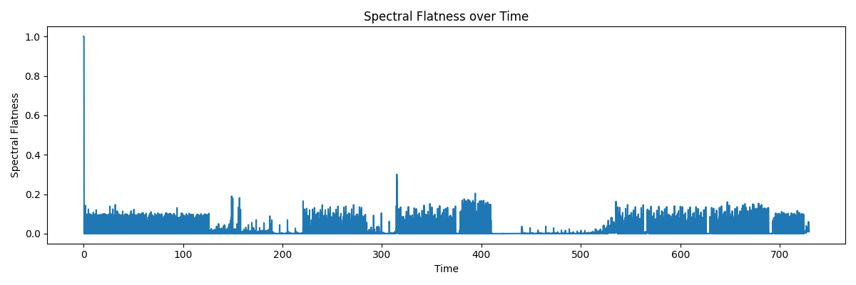
上の図では、普通の楽曲をぶち込んだので、ほとんど値が0に寄っています。

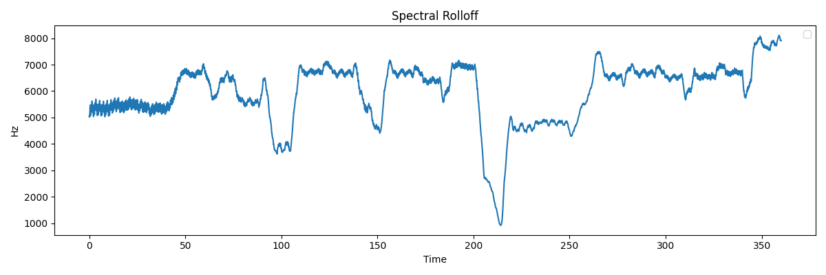
Spectral Rolloff

その時間軸において、スペクトルのエネルギーが全体の85%に達する地点を表します。周波数のある程度の傾向を把握するのに使われたりします。

import librosa
import librosa.display
import matplotlib.pyplot as plt
import numpy as np

y, sr = librosa.load('demo.mp3')
spectral_rolloff = librosa.feature.spectral_rolloff(y=y, sr=sr)[0]
smoothed_data = np.convolve(spectral_rolloff, np.ones(200)/200, mode='valid') # 平滑化
times = librosa.frames_to_time(np.arange(len(smoothed_data)), sr=sr)

plt.figure(figsize=(12, 4))
plt.plot(times, smoothed_data)
plt.ylabel('Hz')
plt.xlabel('Time (seconds)')
plt.title('Spectral Rolloff')
plt.legend(loc='upper right')
plt.tight_layout()
plt.show()

Poly Features

入力された周波数ドメイン(スペクトログラム,mfcc等)を、orderで指定された多項式に変換します。例えば、orderが2の場合の多項式は、$p(x) = ax^2 + bx + c$、orderが3の場合の多項式は、 $p(x) = ax^3 + bx^2 + cx + d$という具合です。

主に機械学習モデルの入力データとして使われるやつだと思います。多分

import librosa
import matplotlib.pyplot as plt
import numpy as np

y, sr = librosa.load(librosa.ex('trumpet'))
S = np.abs(librosa.stft(y))

p0 = librosa.feature.poly_features(S=S, order=0)
p1 = librosa.feature.poly_features(S=S, order=1)
p2 = librosa.feature.poly_features(S=S, order=2)

fig, ax = plt.subplots(nrows=3, sharex=True, figsize=(12, 8))
times = librosa.times_like(p0)
ax[0].plot(times, p0[0], label='order=0', alpha=0.8)
ax[0].plot(times, p1[1], label='order=1', alpha=0.8)
ax[0].plot(times, p2[2], label='order=2', alpha=0.8)
ax[0].legend()
ax[0].label_outer()
ax[0].set(ylabel='Constant term ') # 定数項
ax[1].plot(times, p1[0], label='order=1', alpha=0.8)
ax[1].plot(times, p2[1], label='order=2', alpha=0.8)
ax[1].set(ylabel='Linear term') # 1次項
ax[1].label_outer()
ax[1].legend()
ax[2].plot(times, p2[0], label='order=2', alpha=0.8)
ax[2].set(ylabel='Quadratic term') # 2次項
ax[2].legend()

plt.show()

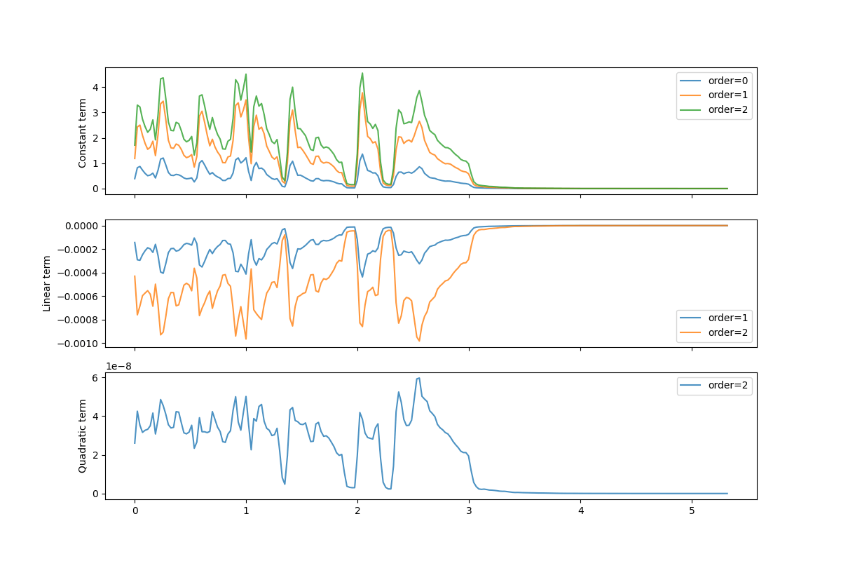
上の図は、トランペット音のpoly_featuresの結果として、上から定数項、1次項、2次項をプロットしています。

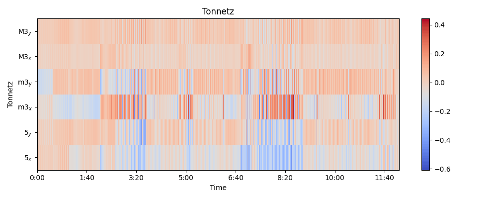
Tonnetz

音楽の和音構造の分析するやつです。音楽理論わからないので説明難しいですが、
Fifth x-axis, Fifth y-axis, Minor x-axis, Minor y-axis, Major x-axis, Major y-axisの6つの和音との各時間軸での適合度を計算するらしいです。
tonnnetz自体は古くから存在する理論で、wikipediaのページがあります。

import librosa
import librosa.display
import matplotlib.pyplot as plt

y, sr = librosa.load('demo.mp3')
harmonic = librosa.effects.harmonic(y)
chroma = librosa.feature.chroma_cqt(y=harmonic, sr=sr)
tonnetz = librosa.feature.tonnetz(y=harmonic, sr=sr, chroma=chroma)

plt.figure(figsize=(10, 4))
librosa.display.specshow(tonnetz, y_axis='tonnetz', x_axis='time')
plt.colorbar()
plt.title('Tonal Centroids (Tonnetz)')
plt.tight_layout()
plt.show()

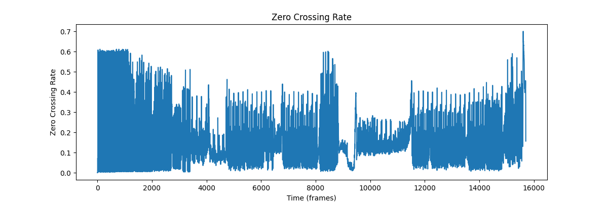
Zero-crossing Rate

信号が正から負、または負から正に切り替わる頻度を計測します。要するに、波形の上下する頻度が多ければ多いほど、値が高くなります。

基本的に、音信号は周波数が高いと波長が短くなるので、Zero-Crossing Rateが高いということは、高い周波数を含むことを意味します。

import librosa
import librosa.display
import matplotlib.pyplot as plt

y, sr = librosa.load('demo.mp3')
zcr = librosa.feature.zero_crossing_rate(y)[0]

plt.figure(figsize=(12, 4))
plt.plot(zcr)
plt.title('Zero Crossing Rate')
plt.xlabel('Time (frames)')
plt.ylabel('Zero Crossing Rate')
plt.show()

ふりかえり

最後の方になるにつれ説明が雑になってしまった。反省。