Benchmark Measurements using Quantum State Tomography on 127-qubit IBM

この記事はJij Inc. Advent Calendar 2023の17日目の記事です。

株式会社JijのHuangです。

本記事では、127量子ビットのIBMデバイスを使用した量子状態トモグラフィーによるベンチマーク測定について考えています。よろしくお願いします。

---

Introduction

In this tutorial, we explore the application of Quantum State Tomography (QST) for benchmark measurements on IBM's latest quantum devices. QST, a experimentally method in quantum computing, allows for the reconstruction of a quantum system's state based on data, playing a crucial role in verifying unknown quantum states^[1]. IBM's 127-qubit quantum devices present an ideal platform for these measurements, offering insights into their capabilities and guiding future enhancements in the field.

Quantum State Tomography^[1:1]

Quantum State Tomography (QST) is an essential tool in quantum information science for experimentally determining an unknown quantum state. QST is the process of reconstructing the quantum state of a system, typically represented by a density matrix, denoted as $\rho$, from experimental measurements.

To be noticed that if we have only a single copy of an unknown quantum state $\rho$, it's impossible to fully characterize it. This limitation arises because there is no quantum measurement can distinguish non-orthogonal states.

Below, we explain the concept and mathematics of QST. For a single qubit density matrix ρ, it can be represented as:

$$\rho = \frac{\rm{tr}(\rho)I + \rm{tr}(X\rho)X + \rm{tr}(Y\rho)Y + \rm{tr}(Z\rho)Z}2$$

,where $\rm{I}$ is the identity matrix, $\rm{X}, \rm{Y}, \rm{Z}$ are Pauli matrices, and $\rm{tr}$ denotes the trace operation.

Then the experimental procedure we will follow includes two parts:

1. Measuring Observables: To estimate terms like $\rm{tr}(Z\rho)$, the observable $Z$ is measured a large number of times. By a similar method, $\rm{tr}(X\rho)$ and $\rm{tr}(Y\rho)$ are estimated. The average values of these observables can be derived from executing the quantum circuit.

2. Estimating Density Matrix: With a sufficiently large number of samples, these measurements provide a reliable estimate of the density matrix $\rho$. This step is crucial for accurately reconstructing the quantum state.

For systems with more than one qubit, an arbitrary density matrix on $n$ qubits can be expanded in a similar way. Measurements of observables, which are products of Pauli matrices, allow the estimation of each term in the sum.

New IBM Quantum Devices

IBM's latest quantum devices are the 127-qubit system, which is now available to open plan users. These devices are named ibm_osaka, ibm_kyoto, and ibm_brisbane. For more detailed specifications of these devices, users can refer to the Compute Resources section on the IBM Quantum Platform.

In this note, we specifically utilize the ibm_osaka device for all our experiments conducted in December 2023.

We provide a demonstration on how to set up the backend using Qiskit.

from qiskit_ibm_runtime import QiskitRuntimeService

service = QiskitRuntimeService(
    channel='ibm_quantum',
    instance='ibm-q/open/main',
    token='Put_your_token'
)

backend = service.backend("ibm_osaka")

Conducting Quantum State Tomography

Quantum state tomography (QST) on IBM's quantum devices can be conducted using the qiskit_experiments.library. QST aims to reconstruct the density matrix of a quantum state through repeated preparation and measurement in a tomographically complete basis. The qiskit_experiments.library facilitates this process, allowing users to operate the necessary measurements and manage data for reconstructing the quantum state.

We offer a detailed demonstration on preparing inputs for State Tomography and executing it using the qiskit_experiments.library.

import qiskit
from qiskit_experiments.framework import ParallelExperiment
from qiskit_experiments.library import StateTomography

# prepare the 0,1,+,R state
qc_0 = qiskit.QuantumCircuit(1)
qc_0.to_instruction()

qc_1 = qiskit.circuit.library.XGate()
qc_p = qiskit.circuit.library.HGate()

qc_r = qiskit.QuantumCircuit(1)
qc_r.h(0)
qc_r.s(0)
qc_r.to_instruction()

state_list = [qc_0, qc_1, qc_p, qc_r]
State_Fidelity_list = []
DensityMatrix_list = []
qubit_index = []
flag = 0

# execute the QST
for state in state_list:
    State_Fidelity_sub_list = []
    DensityMatrix_sub_list = []

    # dicide the physical_qubits from 0 to Q15
    for i in range(0, 16):
        qstexp = StateTomography(state, physical_qubits=[i])
        qstdata = qstexp.run(backend).block_for_results()
        State_Fidelity_sub_list.append(qstdata.analysis_results("state_fidelity").value)
        DensityMatrix_sub_list.append(qstdata.analysis_results("state").value)
        if flag == 0:
            qubit_index.append(qstdata.analysis_results("state").device_components)
    flag = 1
    State_Fidelity_list.append(State_Fidelity_sub_list)
    DensityMatrix_list.append(DensityMatrix_sub_list)

As of December 2023, it's important to note that due to limitations in usage credits, we were unable to test all 127 qubits of the ibm_osaka device.

Additionally, a specific imperfection was identified in qubit Q16, which has been causing errors during the execution of QST. Furthermore, users can visually check the qubit layout and status on the IBM Quantum Platform. The following image, a snapshot taken on December 15, 2023, clearly illustrates the issue. It reveals that not only Q16, but also Q33 and Q106.

The error shows like:

TranspilerError: "HighLevelSynthesis was unable to synthesize Instruction(name='measure', num_qubits=1, num_clbits=1, params=[])."

Analyzing the Results

After successfully conducting QST and collecting state fidelity data, the next crucial step is to analyze these results. An insightful way to present and interpret the data is through visualizations such as graphs.

import matplotlib.pyplot as plt
import numpy as np

data = State_Fidelity_list

# Labels for the groups (assuming they are 0, 1, '+', 'R')
labels = ["0", "1", "+", "R"]

# Indices representing qubits
qubits = np.arange(len(data[0]))  # Assuming qubit indices start from 0
qubit_labels = [f"Q{i}" for i in qubits]

# Plotting the data
plt.figure(figsize=(10, 6))

for i, fidelity in enumerate(data):
    plt.plot(qubit_labels, fidelity, marker="o", label=f"State {labels[i]}")

plt.xlabel("Qubit Index")
plt.ylabel("Fidelity")
plt.title("Fidelity Measurements for Different Qubits")
plt.xticks(qubits)
plt.legend()
plt.grid(True)
plt.show()

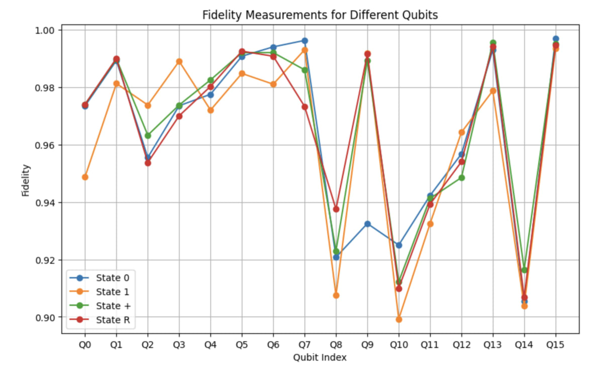
Here is the table presenting the average state fidelity obtained from our results. This table includes detailed data and measurements from our experiments. And we can caculate the total avergae state fidelity: $0.964757825$.

	Average State Fidelity
$\ket{0}$	$0.9639375 \pm 0.0295696$
$\ket{1}$	$0.9621719 \pm 0.0322939$
$\ket{+}$	$0.9671563 \pm 0.0285673$
$\ket{R}$	$0.9657656 \pm 0.0284545$

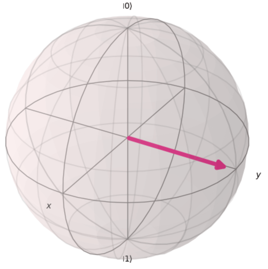
Here, we also can show the experimental state on the Bloch sphere. We have a experimental state and its corresponding density matrix $\rho_{\rm{exp}}$, which can represnt as

$$\rho_{\rm{exp}} = \begin{bmatrix} a & b \\ c & d \end{bmatrix}.$$

Then, let's consider a Bloch vector represented by coordinates $\vec{B}=(x,y,z)$. This vector corresponds to the density operator $\rho$:

$$\rho = \frac{I + xX + yY + zZ}2 = \frac12\begin{bmatrix} 1+z & x-iy \\ x+iy & 1-z \end{bmatrix},$$

where $X,Y,Z$ are Pauli matrices.
Therefore, we establish the relationship between the $\rho_{\rm{exp}}$ and $\vec{B}$:

$$x = 2\,\mathrm{Re}(c) \\ y = 2\,\mathrm{Im}(c) \\ z = 2a - 1.$$

Through this visualization, it is possible to find the differences between ideal $\ket{R}$ state and the actual experimental results. These differences can be caused to various factors, such as device noise or system imperfections, which affect the quantum state during the experiment.

from qiskit.visualization import plot_bloch_vector

def toBloch(matrix):
    [[a, b], [c, d]] = matrix
    x = complex(c).real*2
    y = complex(c).imag*2
    z = complex(2*a-1).real
    return x, y, z

 # change the [3][0] to any [qubit_state][qubit_index]      
plot_bloch_vector(toBloch(DensityMatrix_list2[3][0].data))

Conclusion

In conclusion, we have introduced and demonstrated quantum state tomography using IBM's ibm_osaka quantum devices. Our findings show an average state fidelity of $0.964757825$ across qubits Q0 to Q15. Remarkably, for some qubits, the fidelity even reached as high as 0.99.

Looking forward, it's fascinating to consider further explorations in quantum computing, such as employing quantum process tomography or quantum state transfer. These advanced techniques, noted in references ^[2] and ^[3], have been instrumental in benchmarking quantum processors in past research. They could serve as valuable benchmarks for assessing the performance of the 127-qubit system as well.

最後に

＼Rustエンジニア・数理最適化エンジニア募集中！／

株式会社Jijでは、数学や物理学のバックグラウンドを活かし、量子計算と数理最適化のフロンティアで活躍するRustエンジニア、数理最適化エンジニアを募集しています！
詳細は下記のリンクからご覧ください。皆さんのご応募をお待ちしております！
Rustエンジニア: https://open.talentio.com/r/1/c/j-ij.com/pages/51062
数理最適化エンジニア: https://open.talentio.com/r/1/c/j-ij.com/pages/75132

脚注

1. Nielsen, M. A., & Chuang, I. L. (2010). Quantum computation and quantum information. Cambridge university press.

2. Huang, W. H., Chen, S. H., Chang, C. H., Hsu, T. L., Wang, K. J., & Li, C. M. (2023). Quantum correlation generation capability of experimental processes. Advanced Quantum Technologies, 6(10), 2300113.

3. Huang, Y. T., Lin, J. D., Ku, H. Y., & Chen, Y. N. (2021). Benchmarking quantum state transfer on quantum devices. Physical Review Research, 3(2), 023038.