GET_QUERY_OPERATOR_STATS 最速解説
この記事は Snowflake Advent Calendar 2022 の 20 15 日目です。
はじめに
12 月 16 日頃にリリースされたバージョン 6.41.2 にて、GET_QUERY_OPERATOR_STATS というテーブル関数が Public Preview として追加されました。
このテーブル関数は、History (履歴) ページからアクセスできる各クエリの Profile (プロファイル) 画面に表示されている各操作の統計情報などに SQL からアクセスすることができる、という機能になります。
つまり、今まではクエリプロファイルの情報は GUI から確認することしかできませんでしたが、この関数の追加によりプログラマティックに取得することができるようになりました。
この記事では、GET_QUERY_OPERATOR_STATS 関数と Profile 画面の対応関係や、ちょっとしたサンプルなども交えて解説していきます。
前提
今回は、クエリプロファイルを見るサンプルクエリとして、下記のドキュメントに記載されている TPC-DS の Query57 を使用します:
TPC-DS Query57
use schema snowflake_sample_data.tpcds_sf10tcl;

with v1 as(
  select i_category, i_brand, cc_name, d_year, d_moy,
        sum(cs_sales_price) sum_sales,
        avg(sum(cs_sales_price)) over
          (partition by i_category, i_brand,
                     cc_name, d_year)
          avg_monthly_sales,
        rank() over
          (partition by i_category, i_brand,
                     cc_name
           order by d_year, d_moy) rn
  from item, catalog_sales, date_dim, call_center
  where cs_item_sk = i_item_sk and
       cs_sold_date_sk = d_date_sk and
       cc_call_center_sk= cs_call_center_sk and
       (
         d_year = 1999 or
         ( d_year = 1999-1 and d_moy =12) or
         ( d_year = 1999+1 and d_moy =1)
       )
  group by i_category, i_brand,
          cc_name , d_year, d_moy),
v2 as(
  select v1.i_category ,v1.d_year, v1.d_moy ,v1.avg_monthly_sales
        ,v1.sum_sales, v1_lag.sum_sales psum, v1_lead.sum_sales nsum
  from v1, v1 v1_lag, v1 v1_lead
  where v1.i_category = v1_lag.i_category and
       v1.i_category = v1_lead.i_category and
       v1.i_brand = v1_lag.i_brand and
       v1.i_brand = v1_lead.i_brand and
       v1.cc_name = v1_lag.cc_name and
       v1.cc_name = v1_lead.cc_name and
       v1.rn = v1_lag.rn + 1 and
       v1.rn = v1_lead.rn - 1)
select  *
from v2
where  d_year = 1999 and
        avg_monthly_sales > 0 and
        case when avg_monthly_sales > 0 then abs(sum_sales - avg_monthly_sales) / avg_monthly_sales else null end > 0.1
order by sum_sales - avg_monthly_sales, 3
limit 100;
今回私の環境でこれを実行したときのクエリ ID は 01a8ff70-0000-a6a9-0000-3f8100809252 だったので、このクエリ ID を元に GET_QUERY_OPERATOR_STATS 関数の解説をしていきます。

取得できる情報
今回リリースされた GET_QUERY_OPERATOR_STATS 関数は、前述のように各操作の統計情報を取得するための関数になっています。
すなわち、クエリプロファイル上で各操作、例えば TableScan [0] のようなボックスを選択したときに、右側に出てくる情報が取得できる、という機能になります。
そのため、クエリプロファイルの画面を開いたときに表示されている Profile Overview の情報を取得する機能はまだ Public Preview になっておらず、追って追加される予定になっているので、しばしお待ちください。
まず、クエリプロファイル画面との対応関係を見ていく前に、GET_QUERY_OPERATOR_STATS 関数の結果の各カラムが何を表しているのかを見ていきます。
QUERY_ID
対象のクエリ ID、つまり引数と同じ値が返ります。
STEP_ID
当該行の実行ステップ ID です。
例えば、クエリ実行のリトライが発生した場合や、定数になるサブクエリを含むクエリなど複数ステップでクエリが実行される場合に、複数の STEP_ID が存在する可能性があります。
上記の状況以外では、基本的に常に 1 です。
OPERATOR_ID
各操作 (ノード) の ID です。
注意しなければいけないのは、この OPERATOR_ID は GUI のクエリプロファイルの操作についている番号とまったく一致しません。
例えば、GUI のクエリプロファイルで TableScan[0] と表示されていても OPERATION_ID は 0 ではない可能性があります。
そのため、クエリプロファイルと GET_QUERY_OPERATOR_STATS 関数の結果を紐付ける場合、OPERATOR_ID 以外の情報、例えば OPERATOR_ATTRIBUTES に含まれるオブジェクト名などで同一のものかを確認する必要があります。
PARENT_OPERATOR_ID
その操作の 次の操作の ID です。
Snowflake の実行計画は DAG (有向非巡回グラフ) になっているので、この PARENT_OPERATOR_ID をたどることで DAG を再現することができます。
注意点として、この関数では終点 (SELECT クエリであれば Result) を 0 として処理順とは逆向きに OPERATOR_ID を払い出しており、PARENT_OPERATOR_ID も処理順とは逆向き、すなわち、矢印の向き先である次の操作を「親」としています。
つまり、各操作の前の操作、すなわち各操作の入力行となる操作は、「その操作の OPERATOR_ID を PARENT_OPERATOR_ID カラムに持つ操作」を探す形となります。
…といってもあまりイメージがつきにくいかとは思うので、後述の「おまけ」セクションで具体的な例について解説します。
OPERATOR_TYPE
操作の種類、すなわち TableScan, Join, Aggregate などになります。
これについては、下記ドキュメントの Usage Notes セクションにリストがあるので、そちらを参照してみてください。
OPERATOR_STATISTICS
各操作の統計情報を格納した JSON オブジェクトとなっており、内容は OPERATOR_TYPE によって異なりますが、その操作に入力された行数 (操作対象となった行数) である input_rows はすべての OPERATOR_TYPE で存在します。
それぞれの操作でどのような統計情報が取得できるかについては、下記ドキュメントの OPERATOR_STATISTICS セクションにリストがあるので、そちらを参照してみてください。
EXECUTION_TIME_BREAKDOWN
各操作内における各処理の実行時間の内訳(例外あり)を、比率 (0〜1) の値とともに格納した JSON オブジェクト……なのですが、このカラムの値の読み方は少々複雑になっています。
まず値の種類についてですが、OPERATOR_TYPE にかかわらず、すべての行に overall_percentage という行が存在し、これは「各操作内における各処理の実行時間の内訳」ではなく「クエリ全体における当該操作の実行時間の内訳」を表す比率となります。これが上記の「例外」です。
すなわち、GET_QUERY_OPERATOR_STATS 関数の結果のすべての overall_percentage を合計すると 1 になります。
この overall_percentage に加えて、OPERATOR_TYPE によっては「操作内の各処理の実行時間の内訳」の取得に対応しているものがあり、overall_percentage 以外の複数の項目が存在する場合があります。
…がここからが複雑なポイントで、overall_percentage 以外の項目を合計しても 1 にはなりません。 代わりに、overall_percentage 以外の項目を合計すると overall_percentage の値になります。
したがって「各操作内における各処理の実行時間の内訳」の合計が 1 (100%) になるようにするためには、overall_percentage 以外の各項目を overall_percentage で割ってあげる必要がある点に注意してください。
後述の「クエリプロファイル画面との対応関係」セクションで、具体的なクエリの例が出てくるので、そちらも参考に確認してみてください。
また、各項目の詳細については EXECUTION_TIME_BREAKDOWN セクションにリストがあるので、そちらを参照してみてください。
OPERATOR_ATTRIBUTES
各操作に関する付加情報、例えば Join であれば結合条件や結合タイプ、TableScan であれば対象のテーブル名などを格納した JSON オブジェクトとなっており、OPERATOR_TYPE によっては空の場合もあります。
それぞれの操作にどのような付加情報が取得できるかについては、下記ドキュメントの OPERATOR_ATTRIBUTES セクションにリストがあるので、そちらを参照してみてください。
クエリプロファイル画面との対応関係
以下では、各操作を選択したときに表示されるそれぞれのボックスが、どのように GET_QUERY_OPERATOR_STATS 関数を使用したクエリに対応しているかを解説していきます。
Node Execution Time
クエリプロファイル画面の Node Execution Time は、
- この操作 (ノード) が、クエリ全体の実行時間に対して何 % を占めるか
- この操作の実行時間に対して、各処理が何 % を占めるか
という 2 つの情報で EXECUTION_TIME_BREAKDOWN カラムの情報に一致します。

Classic Web Interface

Snowsight
例えば、上記の画像は SNOWFLAKE_SAMPLE_DATA.TPCDS_SF10TCL.CATALOG_SALES テーブルに対する TableScan の Node Execution Time になるので、下記のようなクエリで同じ情報を GET_QUERY_OPERATOR_STATS 関数から取得することができます。
select
    operator_attributes:table_name::varchar "Table",
    round(execution_time_breakdown:overall_percentage*100, 1) "Node Execution Time",
    round(execution_time_breakdown:processing/execution_time_breakdown:overall_percentage*100, 1) "Processing",
    round(execution_time_breakdown:local_disk_io/execution_time_breakdown:overall_percentage*100, 1) "Local Disk I/O",
    round(execution_time_breakdown:remote_disk_io/execution_time_breakdown:overall_percentage*100, 1) "Remote Disk I/O",
    round(execution_time_breakdown:network_communication/execution_time_breakdown:overall_percentage*100, 1) "Network Communication",
    round(execution_time_breakdown:synchronization/execution_time_breakdown:overall_percentage*100, 1) "Synchronization",
from table(get_query_operator_stats('01a8ff70-0000-a6a9-0000-3f8100809252'))
where operator_type = 'TableScan'
and operator_attributes:table_name::varchar = 'SNOWFLAKE_SAMPLE_DATA.TPCDS_SF10TCL.CATALOG_SALES'
;
/*
Table	Node Execution Time	Processing	Local Disk I/O	Remote Disk I/O	Network Communication	Synchronization
SNOWFLAKE_SAMPLE_DATA.TPCDS_SF10TCL.CATALOG_SALES	83.3	2	0	81	0	0
*/
ここで重要なポイントが "Node Execution Time" 以外のすべての項目について execution_time_breakdown:overall_percentage で割っている部分になります。
ここがまさに「取得できる情報」セクションで前述した「overall_percentage 以外の項目を合計すると overall_percentage の値になる」という動作を調整している部分で、割ってあげることで合計が 1 (100%) になり、クエリプロファイルの表示と一致する形となります。
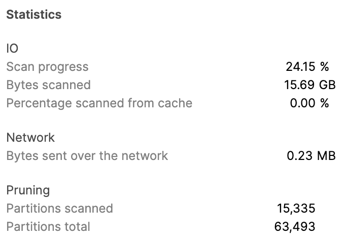
Statistics
クエリプロファイル画面の Statistics は各操作ごとの統計情報で OPERATOR_STATISTICS カラムの情報に一致します。
Classic Web Interface

Snowsight
上記の画像は、同じく SNOWFLAKE_SAMPLE_DATA.TPCDS_SF10TCL.CATALOG_SALES テーブルに対する TableScan の Statistics になるので、下記のようなクエリで同じ情報を GET_QUERY_OPERATOR_STATS 関数から取得することができます。
select
    operator_attributes:table_name::varchar "Table",
    round(operator_statistics:io:scan_progress*100, 2) || ' %' "Scan progress",
    format_bytes(operator_statistics:io:bytes_scanned) "Bytes scanned",
    round(operator_statistics:io:percentage_scanned_from_cache*100, 2) || ' %' "Percentage scanned from cache",
    format_bytes(operator_statistics:network:network_bytes) "Bytes sent over the network",
    operator_statistics:pruning:partitions_scanned "Partitions scanned",
    operator_statistics:pruning:partitions_total "Partitions total"
from table(get_query_operator_stats('01a8ff70-0000-a6a9-0000-3f8100809252'))
where operator_type = 'TableScan'
and operator_attributes:table_name::varchar = 'SNOWFLAKE_SAMPLE_DATA.TPCDS_SF10TCL.CATALOG_SALES'
;
/*
Table	Scan progress	Bytes scanned	Percentage scanned from cache	Bytes sent over the network	Partitions scanned	Partitions total
SNOWFLAKE_SAMPLE_DATA.TPCDS_SF10TCL.CATALOG_SALES	24.15 %	15.69 GB	0 %	0.23 MB	15335	63493
*/
FORMAT_BYTES 関数はこんな感じで作った UDF になります:
create or replace function format_bytes (bytes int)
returns varchar
language sql as $$
    case when len(bytes) >= 13 then round(bytes/1024/1024/1024/1024, 2) || ' TB'
         when len(bytes) >= 10 then round(bytes/1024/1024/1024, 2) || ' GB'
         else round(bytes/1024/1024, 2) || ' MB'
    end
$$
;
ちなみに「Scan progress が 24.15 % なのってどういうことなの」という話ですが、これは LIMIT 句があると LIMIT 句に必要な行数が集まるまでとりあえずクエリを実行し続けて、集まったところでクエリ実行打ち切るように動作するので、打ち切られたタイミングでどれぐらいテーブルスキャンが完了していたかを表しています。
つまり、今回のケースでは 100 行の結果が集まるまでに、スキャン対象データのうち 24.15 % が読み込まれたことになります。
Attributes
クエリプロファイル画面の Attributes は各操作ごとの付加情報で OPERATOR_ATTRIBUTES カラムの情報に一致します。

Classic Web Interface

Snowsight
上記の画像は、同じく SNOWFLAKE_SAMPLE_DATA.TPCDS_SF10TCL.CATALOG_SALES テーブルに対する TableScan の Attributes になるので、下記のようなクエリで同じ情報を GET_QUERY_OPERATOR_STATS 関数から取得することができます。
select
    operator_attributes:table_name::varchar "Full table name",
    operator_attributes:columns "Columns"
from table(get_query_operator_stats('01a8ff70-0000-a6a9-0000-3f8100809252'))
where operator_type = 'TableScan'
and operator_attributes:table_name::varchar = 'SNOWFLAKE_SAMPLE_DATA.TPCDS_SF10TCL.CATALOG_SALES'
;
/*
Full table name	Columns
SNOWFLAKE_SAMPLE_DATA.TPCDS_SF10TCL.CATALOG_SALES	[ "CS_SOLD_DATE_SK", "CS_CALL_CENTER_SK", "CS_ITEM_SK", "CS_SALES_PRICE" ]
*/
実用例
Spill
Spill は、テーブルスキャン、結合、集約、ソートなどに必要なメモリ容量が足りない場合に、通常、メモリ上に作成される一時領域をストレージに書き出して処理することを指します。
下記ドキュメントの「クエリプロファイルによって識別される一般的なクエリの問題」セクションにある「大きすぎてメモリに収まらないクエリ」サブセクションが、まさに Spill が発生している状況です。
上記のドキュメントに記述されているように、Spill は 2 段階で発生し、まずメモリが足りなくなるとローカルストレージ (仮想ウェアハウスサーバのインスタンスストア) に書き出され、ローカルストレージも足りなくなるとリモートストレージ (S3 などのオブジェクトストレージ) に書き出されます。
ストレージ I/O はメモリ I/O よりも圧倒的に遅いので、Spill の発生はパフォーマンス低下の大きな原因となり、特にリモートストレージ I/O は API 経由での HTTPS のダウンロード/アップロードになるため、急激なパフォーマンス低下の原因となります。
Spill が発生しているかどうかは、以前も QUERY_HISTORY ビューの BYTES_SPILLED_TO_LOCAL_STORAGE および BYTES_SPILLED_TO_REMOTE_STORAGE カラムで確認することができましたが、どの処理で Spill が発生しているかを特定するためにはクエリプロファイルを確認する必要がありました。
しかし GET_QUERY_OPERATOR_STATS 関数を使用すると、これを SQL で確認することができるようになります。
今回は TPC-DS 10TB の CUSTOMER テーブル (6,500 万行 / 2.9 GB) を XSMALL 仮想ウェアハウス上でソートするクエリで検証してみます。
create or replace warehouse temp warehouse_size = xsmall;

select *
from snowflake_sample_data.tpcds_sf10tcl.customer
order by c_first_sales_date_sk
;

select last_query_id();
-- 01a904a0-0000-a74e-0000-3f81008145e2
Spill の情報は Spill が発生した場合のみ OPERATOR_STATISTICS カラムの spilling 項目として出現します。
すなわち、Spill が発生していない操作では operator_statistics:spilling:bytes_spilled_local_storage が NULL になり、NULL 値との比較は常に NULL になるため、
operator_statistics:spilling:bytes_spilled_local_storage > 0operator_statistics:spilling:bytes_spilled_local_storage is not null
のような WHERE 句条件でフィルタすることで、実際に Spill が発生している操作のみが表示され、原因を特定することができます。
select
    operator_type,
    operator_attributes,
    nvl(operator_statistics:spilling:bytes_spilled_local_storage, 0) spill_local_raw,
    nvl(operator_statistics:spilling:bytes_spilled_remote_storage, 0) spill_remote_raw,
    format_bytes(spill_local_raw) spill_local,
    format_bytes(spill_remote_raw) spill_remote
from table(get_query_operator_stats('01a904a0-0000-a74e-0000-3f81008145e2'))
where spill_local_raw > 0
order by spill_remote_raw, spill_local_raw
;
/*
OPERATOR_TYPE	OPERATOR_ATTRIBUTES	SPILL_LOCAL_RAW	SPILL_REMOTE_RAW	SPILL_LOCAL	SPILL_REMOTE
Sort	{ "sort_keys": [ "CUSTOMER.C_FIRST_SALES_DATE_SK ASC NULLS LAST" ] }	5098991616	0	4.75 GB	0.00 MB
*/
ちなみに Spill が発生していたときの対応策は大きく
- メモリ容量を増やす = より大きい仮想ウェアハウスサイズを使用する
- Spill が発生している操作に入力されるデータ量・行数を減らす
- 先出しできる集約を先出しする
- WHERE 句の条件を追加・変更する
- 不要なカラム・テーブルをクエリから削除する
などになるため、もし Spill が問題になっていることが確認できた場合には、参考にしてみてください。
Join Explosion
Join Explosion (結合爆発) は、結合の左右それぞれのテーブルの行数)に対して結合結果の行数が急激に大きくなってしまっている状況のことです。
Join Explosion が発生していると、その結合以降の中間行数が多くなり、後続の集約やソート、ウィンドウ関数などの「行数に相関して遅くなる操作」の処理時間に大きな影響を与えてしまいます。
この事象は、実行計画生成がうまく行かなかった場合や、結合条件が一対多で対応する場合、クロス結合や、選択性の低い結合フィルタを含むクエリなどで発生します。
Join Explosion が発生しているかどうかは、Spill の場合と同じように、今まではクエリプロファイル画面で各結合の入力行数と出力行数を確認するしかありませんでしたが、GET_QUERY_OPERATOR_STATS 関数を使用すると、これを SQL で確認することができるようになった上に、複雑なクエリであっても簡単に一覧で並べて確認することができるようになりました。
今回は、以下のようなクエリで検証してみます。
create or replace table t1 (c1 int) as
select seq4()%10
from table(generator(rowcount => 10000))
;

create or replace table t2 (c1 int) as
select seq4()%100
from table(generator(rowcount => 10000))
;

create or replace table t3 (c1 int) as
select seq4()%1000
from table(generator(rowcount => 10000))
;

create or replace table t4 (c1 int) as
select seq4()%10000
from table(generator(rowcount => 10000))
;

select *
from t1
join t2 on t1.c1 = t2.c1
join t3 on t1.c1 = t3.c1
join t4 on t1.c1 = t4.c1
;
このクエリでは、t1, t2, t3, t4 がそれぞれ 10, 100, 1000, 10000 種類の値を持っているので、t1.c1 = t2.c1 はかなり重複行が存在していて、t1.c1 = t4.c1 はほとんど重複行がないことが想定されます。
結果としては、下記のようになり、想定と一致します。
select
    operator_id,
    operator_statistics:input_rows input_rows,
    operator_statistics:output_rows output_rows,
    round(output_rows/input_rows, 2) magnification,
    operator_attributes:equality_join_condition::varchar join_keys,
    operator_attributes:additional_join_condition::varchar post_join_filters,
    operator_attributes:join_type::varchar join_type
from table(get_query_operator_stats(last_query_id()))
where operator_type = 'Join'
order by magnification desc, output_rows desc
;
/*
OPERATOR_ID	INPUT_ROWS	OUTPUT_ROWS	MAGNIFICATION	JOIN_KEYS	POST_JOIN_FILTERS	JOIN_TYPE
1	110000	10000000	90.91	(T2.C1 = T1.C1)		INNER
3	20000	100000	5	(T3.C1 = T1.C1)		INNER
5	11000	10000	0.91	(T4.C1 = T1.C1)		INNER
*/
T4.C1 = T1.C1 の input_rows が 11000 になっているのが少々不思議ですが、これは Join Filter と呼ばれる結合条件ベースの実行時プルーニングの結果、t4 の行のうち 1,000 行だけしか読み込まなくていいと判断されたためとなります。
具体的には T4.C1 = T1.C1 以外の結合の結果を考えると、含まれる値の数は最大でも t3 に含まれる 1,000 種類になり、内部結合である以上それ以外の行が結果に含まれることはないので、t4 からはその 1,000 行しか読む必要がないから残りの 9,000 行は読まない、という判断になります。
おまけ
Recursive CTE で DAG をたどってみる
OPERATOR_ID と PARENT_OPERATOR_ID を結合条件にすることで、Recursive CTE を使って再帰的に DAG をたどることができます。
このとき、前述のように最後のノードが根 (PARENT_OPERATOR_ID が NULL) になるので、最後のノードから逆順にたどっていく必要があります。
with
operators as (
    select operator_id, parent_operator_id, operator_type
    from table(get_query_operator_stats('01a8ff70-0000-a6a9-0000-3f8100809252'))
),
graph_recursive as (
    select operator_id, parent_operator_id, operator_type path
    from operators
    where parent_operator_id is null -- root
    union all
    select o.operator_id, o.parent_operator_id, g.path || ' <- ' || o.operator_type
    from graph_recursive g
    join operators o on g.operator_id = o.parent_operator_id
)
select path
from graph_recursive
order by path
;
結果はこんな感じになります。
実行結果
PATH
Result
Result <- SortWithLimit
Result <- SortWithLimit <- Join
Result <- SortWithLimit <- Join <- Filter
Result <- SortWithLimit <- Join <- Filter <- JoinFilter
Result <- SortWithLimit <- Join <- Filter <- JoinFilter <- WithReference
Result <- SortWithLimit <- Join <- Join
Result <- SortWithLimit <- Join <- Join <- Filter
Result <- SortWithLimit <- Join <- Join <- Filter
Result <- SortWithLimit <- Join <- Join <- Filter <- JoinFilter
Result <- SortWithLimit <- Join <- Join <- Filter <- JoinFilter <- WithReference
Result <- SortWithLimit <- Join <- Join <- Filter <- WithReference
Result <- SortWithLimit <- Join <- Join <- Filter <- WithReference <- WithClause
Result <- SortWithLimit <- Join <- Join <- Filter <- WithReference <- WithClause <- WindowFunction
Result <- SortWithLimit <- Join <- Join <- Filter <- WithReference <- WithClause <- WindowFunction <- Aggregate
Result <- SortWithLimit <- Join <- Join <- Filter <- WithReference <- WithClause <- WindowFunction <- Aggregate <- Aggregate
Result <- SortWithLimit <- Join <- Join <- Filter <- WithReference <- WithClause <- WindowFunction <- Aggregate <- Aggregate <- Join
Result <- SortWithLimit <- Join <- Join <- Filter <- WithReference <- WithClause <- WindowFunction <- Aggregate <- Aggregate <- Join <- Aggregate
Result <- SortWithLimit <- Join <- Join <- Filter <- WithReference <- WithClause <- WindowFunction <- Aggregate <- Aggregate <- Join <- Aggregate <- Join
Result <- SortWithLimit <- Join <- Join <- Filter <- WithReference <- WithClause <- WindowFunction <- Aggregate <- Aggregate <- Join <- Aggregate <- Join <- Aggregate
Result <- SortWithLimit <- Join <- Join <- Filter <- WithReference <- WithClause <- WindowFunction <- Aggregate <- Aggregate <- Join <- Aggregate <- Join <- Aggregate <- Join
Result <- SortWithLimit <- Join <- Join <- Filter <- WithReference <- WithClause <- WindowFunction <- Aggregate <- Aggregate <- Join <- Aggregate <- Join <- Aggregate <- Join <- Filter
Result <- SortWithLimit <- Join <- Join <- Filter <- WithReference <- WithClause <- WindowFunction <- Aggregate <- Aggregate <- Join <- Aggregate <- Join <- Aggregate <- Join <- Filter
Result <- SortWithLimit <- Join <- Join <- Filter <- WithReference <- WithClause <- WindowFunction <- Aggregate <- Aggregate <- Join <- Aggregate <- Join <- Aggregate <- Join <- Filter <- JoinFilter
Result <- SortWithLimit <- Join <- Join <- Filter <- WithReference <- WithClause <- WindowFunction <- Aggregate <- Aggregate <- Join <- Aggregate <- Join <- Aggregate <- Join <- Filter <- JoinFilter <- TableScan
Result <- SortWithLimit <- Join <- Join <- Filter <- WithReference <- WithClause <- WindowFunction <- Aggregate <- Aggregate <- Join <- Aggregate <- Join <- Aggregate <- Join <- Filter <- TableScan
Result <- SortWithLimit <- Join <- Join <- Filter <- WithReference <- WithClause <- WindowFunction <- Aggregate <- Aggregate <- Join <- Aggregate <- Join <- TableScan
Result <- SortWithLimit <- Join <- Join <- Filter <- WithReference <- WithClause <- WindowFunction <- Aggregate <- Aggregate <- Join <- TableScan
*/
ちなみに出力ももっときれいにできるといいのですが、手続き型言語と違って SQL の再帰はすべての子ノードを同時に探索することしかできないので、「葉に到達したらどうこう」みたいな処理を書くのがほぼほぼ不可能なため、これが限界です。
クエリプロファイル画面と同じようなグラフを描いてみる
……というわけで、せっかく Zenn が Mermaid でのグラフ描画に対応しているので、SQL で Mermaid の DSL を生成して、クエリプロファイルのようなグラフを描いてみます。
with
nodes as (
    select
        concat(operator_id, '["', operator_type, '[', operator_id, ']"]') node,
        operator_type,
        operator_id,
        parent_operator_id,
        operator_statistics:input_rows::int input_rows
    from table(get_query_operator_stats($qid))
),
edges as (
    select
        n.operator_id,
        concat(n.node, '-- ', p.input_rows, ' -->', p.node) edge
    from nodes n
    left join nodes p on n.parent_operator_id = p.operator_id
)
select 'flowchart BT\n\t' || listagg(edge, '\n\t') within group (order by operator_id) mermaid_script
from edges
;
結果はこんな感じになります。
flowchart BT
	1["SortWithLimit[1]"]-- 100 -->0["Result[0]"]
	2["Join[2]"]-- 5325679 -->1["SortWithLimit[1]"]
	3["Join[3]"]-- 12669218 -->2["Join[2]"]
	4["Filter[4]"]-- 5325756 -->3["Join[3]"]
	5["TableScan[5]"]-- 77 -->4["Filter[4]"]
	6["Join[6]"]-- 5325756 -->3["Join[3]"]
	7["Filter[7]"]-- 23098977 -->6["Join[6]"]
	8["Aggregate[8]"]-- 750 -->7["Filter[7]"]
	9["Filter[9]"]-- 433390270 -->8["Aggregate[8]"]
	10["WithReference[10]"]-- 437315567 -->9["Filter[9]"]
	11["WithClause[11]"]-- 437315567 -->10["WithReference[10]"]
	12["Aggregate[12]"]-- 437315567 -->11["WithClause[11]"]
	13["Join[13]"]-- 553348851 -->12["Aggregate[12]"]
	14["Filter[14]"]-- 553630693 -->13["Join[13]"]
	15["TableScan[15]"]-- 365 -->14["Filter[14]"]
	16["Filter[16]"]-- 553630693 -->13["Join[13]"]
	17["JoinFilter[17]"]-- 553630328 -->16["Filter[16]"]
	18["TableScan[18]"]-- 553630328 -->17["JoinFilter[17]"]
	19["Filter[19]"]-- 23098977 -->6["Join[6]"]
	20["JoinFilter[20]"]-- 23098267 -->19["Filter[19]"]
	21["WithReference[21]"]-- 437315567 -->20["JoinFilter[20]"]
	22["JoinFilter[22]"]-- 12669218 -->2["Join[2]"]
	23["TableScan[23]"]-- 7343539 -->22["JoinFilter[22]"]
これを Mermaid で描画してみると…
前述のように、クエリプロファイルと各操作の番号は一致しないものの、同じようなグラフを描くことができました。
まとめ
個人的に GET_QUERY_OPERATOR_STATS 関数は Snowflake 運用、特にユーザ側での調査や検証におけるゲームチェンジャーだと思っているので、ぜひ使ってみてください。
現状はまだ Public Preview なので本番環境で使用しないようにしていただきたい機能になりますが、ぜひいろいろ遊んでみて、不具合や改善点などあれば Snowflake Support に連絡してみてください!
Discussion