🐈

MLモデルと解釈性 "Weighted SHAP" 実装と解説

2023/10/03に公開

WeightedSHAP: analyzing and improving Shapley based
Yongchan Kwon, James Zou
NeurIPS 2022
https://arxiv.org/abs/2209.13429

表データを用いた回帰モデルの解釈性について勉強していてSHAPに興味を持ったので、最近NIPSで見たWeightedSHAPをツールとして使うための数式部分を理解して行きます。
図は論文からの引用です。

公式リポジトリ

この論文が言いたいこと

SHAPはMLモデルの予測値を特徴量方面から解釈するときに重要だが、元々ゲーム理論から発展した手法のためMLでは自然ではない公理からくる解釈があり、特に特徴量列にデータの多寡があるとShapley値を求めるときの単純な線形和 $\sum_{j} φ_{j}$ では対応できない。
これに対処するため、WeightedSHAPではShapley値の特徴の帰属(feature attribution)の数学的な解析と、影響力の低い特徴に対してより大きな帰属を割り当てるという最適でない状況を特定し、この洞察を基にShapley値の一般化と、データから直接どの限界貢献にフォーカスするかを学習する手法を提案しており、モデルの予測をよりよく再現(つまりSHAP値による分解が正確に)できるようにした。

例えば線形モデルや決定木は解釈性が高く、回帰係数やノードの条件などから予測値を理解することができるが、最近のDNNやランダムフォレストなどの方法は解釈に関して直感的でない。これをモデルを弄らずに特徴量と推論を使って解釈する方法が[1]のSHapley Additive exPlanations (SHAP)であり、これはShaply値が満たす理論的性質が良いため支持されているが、計算コストの高さはネックである。

元論文の主な貢献点:

SHAPの限界貢献の分析によりShaply値の非最適性を示したこと
柔軟なShaply値の一般化であるWeightedSHAPを提案したこと

Shaply値のただの和を用いた解釈では、異なる限界貢献が異なるシグナル(?)とノイズを持つ場合に帰属誤り(attribution mistakes)を起こすことがあり、これを正すためにデータから加重平均の重みを学習する方法を提案している。
また単純な変更であるため、従来のSHAPの実装からすぐに変更できる。

[1] Scott M Lundberg and Su-In Lee. A unified approach to interpreting model predictions. In Proceedings of the 31st international conference on neural information processing systems, pages 4768-4777, 2017.

そもそもSHAPとは

まず限界貢献とShapley値について振り返る。

入力次元 $d ∈ \mathbb{N}$
入力空間 $\mathcal{X} ⊆ \mathbb{R}^{d}$
出力空間 $\mathcal{Y} ⊆ \mathbb{R}$
確率変数 $X = (X_{1}, \dots X_{d}) ∈ \mathcal{X}$
実現値 $x = (x_{1}, \dots x_{d})$
モデル $\hat{f} : \mathcal{X} → \mathcal{Y}$
集合 $[j] := {1, \dots j}$ とその冪 $2^{[j]}$
ベクトル $u ∈ \mathbb{R}^{d}$ と $S := (j_{1}, \dots j_{|S|} ⊆ [d])$ により表される部分ベクトル $u_{S} := (u_{\substack{j\\1}}, \dots u_{\substack{j\\|S|}})$
$X$ は任意の部分集合 $S ⊊ [d]$ に対して条件付き分布 $p(X_{[d]\backslash S} | X_{S})$ がwell-difinedな同時分布 $p(X)$ を持つとする

以上の前提で、[2]で定義される条件付き提携関数(conditional coalition function) $v^{(\text{cond})}_{x,\hat{f}} : 2^{[d]} → \mathbb{R}$ は次の式で表される。

v^{(\text{cond})}_{x,\hat{f}} (S) := \mathbb{E}[\hat{f}(x_{S}, X_{[d]\backslash S}) | X_{S}=x_{S}] - \mathbb{E}[\hat{f}(X)]

条件付き提携関数 $v^{(\text{cond})}_{x,\hat{f}} (S)$ は、雑に言えば情報量を表しており、無情報の予測値と比較して部分情報 $x_{S}$ を観測した後の予測値がどれだけ回復するかを示している。
ここで $u_{i} = x_{i} \space \texttt{if} (i ∈ S) \texttt{else} \space X_{i}$ とすることで、 $\hat{f}(x_{S}, X_{[d]\backslash S})$ を $\hat{f}(u)$ と簡潔に書く。また $v^{(\text{cond})}_{x,\hat{f}}$ の $x,\hat{f}$ は省略する。

$v^{(\text{cond})} (\empty) := 0$
$v^{(\text{cond})} ([d]) := \hat{f}(x) - \mathbb{E}[\hat{f}(X)]$

上の2つは慣例に従った定義であるが、つまるところ無情報の時は $\mathbb{E}[\hat{f}(x_{S}, X_{[d]\backslash S}) | X_{S}=x_{S}]$ が周辺期待値 $\mathbb{E}[\hat(f)(X)]$ となるため、何も情報量を持たない、予測を回復しないということとなる。

[2] Scott M Lundberg and Su-In Lee. A unified approach to interpreting model predictions. In Proceedings of the 31st international conference on neural information processing systems, pages 4768-4777, 2017.

限界寄与に基づく帰属法(attribution methods)

「SHAPは何をしたいか」について立ち戻ると、予測値 $\hat{f}(x)$ の個々の変数 $x_{i}$ の重要性を割り当てることであり、どのようにして影響力を測定するかを考える必要がある。
まず、ある特徴を1つ追加した後の $v^{cond}$ の差として限界貢献を定量化する。

限界貢献(Marginal contribution) $Δ_{j}(x_{i})$ は、特徴量 $x_{i} | i,j ∈ [d]$ について、提携(coalition)のサイズ(つまり注目している特徴 $i$ 以外の特徴量の数 $|S| = j-1$ ) から取ってこれる全ての部分集合の組み合わせを使って、それに注目している特徴量 ${i}$ を含む場合と含まない場合の $v^{(\text{cond})}$ の差を測った量である。
次のように定義される。

Δ_{j}(x_{i}) := \frac{1}{_{d-1}C_{j-1}} \sum_{\substack{S⊆[d]\backslash \{i\} \\ |S| =j-1}} v^{(\text{cond})}(S ∪ \{i\}) - v^{(\text{cond})}(S)

雑に言うと、 $x_{i}$ 以外の $[j]$ の特徴量のマスクの全組み合わせと、それに $x_{i}$ を加えたものとの差、情報量を平均して評価する計算によって、特徴 $x_{i}$ が部分集合 $S$ に追加されたときの平均寄与度を測定している。

さらに、[3]などで使われるShapley値を用いる方法として次の定義が使える。

φ_{\text{shap}}(x_{i}) := \frac{1}{d} \sum_{j=1}^{d} Δ_{j}(x_{i})

雑に言うと、特徴量 $x_{i}$ の限界貢献を $j = 1 \dots d$ について平均し、特徴量の影響を要約している。

以下は筆者が理解できていない部分であるが雑に訳してメモしておく...

Shaply値は協力ゲーム理論におけるfair divisionの4つの公理を満たす唯一の関数として定義されるが、公理の経済的概念が帰属問題に直感的に適用できないことがあるという重大な問題があるらしい。
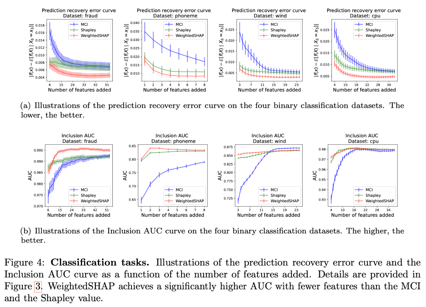
例えば帰属の総和が限界貢献度の中の $v^{\text{(cond)}}([d])$ に等しいことを要求する効率公理は、帰属の順序が定数の乗算に不変であるため必ずしも本質的ではない。任意の正の定数 $C > 0$ に対して、属性 $φ_{C}(x_{i}) := C × φ_{shap}(x_{i})$ はShapley値 $v^{\text{(cond)}}$ と同じ次数を持つが、効率公理は $φ_{C}$ には必要ないとのこと。これに関して元論文では再検討し効率公理を緩和した新しい帰属方法を紹介している。

また、評価指標として包含AUC (area under the receiver operating characteristic curve)がよく知られている。まず帰属値に基づいて特徴がランク付けされ、次にAUCが最も影響力のある特徴から最も影響力のない特徴まで1つずつ追加することによって繰り返し評価されることで、追加した特徴数の関数としてAUC曲線が生成され、包含AUCはこの曲線下の面積として定義される。また同様の評価手法としてAUP (Area under the prediction recovery error curve)も使われている。

入力 $x ∈ \mathcal{X}$
$k \in [d]$
帰属法 $φ(x_j)$ に基づき、最も影響の強い $k$ 個の特徴量に対応する整数を表す集合 $\mathcal{L}(k; φ,x) ⊆ [d]$

\text{APU}(φ; x, \hat{f}) := \sum_{k=1}^{d} | \hat{f}(x) - \mathbb{E}[(\hat{f}(X) | X_{\mathcal{L}(k; φ,x)} = x_{\mathcal{L}(k; φ,x)}]|

[3] Scott M Lundberg and Su-In Lee. A unified approach to interpreting model predictions. In Proceedings of the 31st international conference on neural information processing systems, pages 4768-4777, 2017.

限界貢献の閉形式の式

$\hat{f}$ が線形で $p(X) = N(X | 0_{d}, Σ_{\bold{ρ},\bold{d}}^{(\text{block})})$ である場合の限界寄与を閉形式の式で導出する。
設定は以下。

モデル $\hat{f}$ が線形関数 $\hat{f}(x) = \hat{β}_{0} + x^{\top} \hat{β}$
$(\hat{β}_{0}, \hat{β}) ∈ \mathbb{R} × \mathbb{R}^{d}$
共分散次元 $B ∈ \mathbb{N}$
共分散行列 $Σ_{\bold{ρ},\bold{d}}^{(\text{block})} = \text{diag}(Σ_{\bold{ρ}_{1},\bold{d}_{1}}, \dots Σ_{\bold{ρ}_{B},\bold{d}_{B}})$
$\bold{d} := (d_{1}, \dots d_{B}) ∈ \mathbb{N}^{B}$ ただし $\sum \bold{d} = d$
$\bold{ρ} := (ρ_{1}, \dots ρ_{B}) ∈ [0,1)^{B}$
$Σ_{\bold{ρ}_{b},\bold{d}_{b}} = (1 - ρ_{b}) I_{d_{b}} + ρ_{b} \mathbb{i}_{d_{b}} \mathbb{i}_{d_{b}}^{\top}$
$i\timesi$ 単位行列 $I_{i}$
全要素が1の $i$ 次元ベクトル $\mathbb{i}_{i}$

すなわち、

各特徴は単位分散を持つように正規化されている
各特徴は $B$ 個の独立のクラスタのどれかに含まれる。
例えば $j \in [B]$ の場合 $j$ 番目のクラスタのサイズは $d_{j}$ で、特徴量の相関はクラスタ内で互いに等しい

通常、限界貢献は閉形式の式を持たないが、上記の設定においては限界貢献 $i$ 番目の特徴量 $x_{i}$ の $j-1$ サンプルに対して次の閉形式で表される。

Δ_{j}(x_{i}) = x^{\top} H(i,j) \hat{β}

$i,j \in [d]$
$H(i,j)$ は明示的な行列(元論文の付録に解がある)

この定理は限界貢献が入力 $x$ と推定回帰係数 $\hat{β}$ のbilinearな関数であることを示しており、Shapley値もbilinearになる。

bilinearだと計算効率が劇的に改善するためうれしい。式の通り、 $H(i,j)$ が入力 $x$ と独立なので、1度計算すればよいだけになる。また $H(i,j)$ はメモリに保存しなくてよい(なぜ?)ため、メモリ効率もよい。

最適な帰属が計算できない例

まず $d=2$ の場合に任意の帰属法 $φ$ によりAUPが2つの値しか取らないことを用いて、影響力のある特徴量へ大きな値を割り当てることができない例が存在することを示す。

$\mathcal{E}(k_{=\{1,2\}}; x, \hat{f}) = | \hat{f}(x_1, x_2) - \mathbb{E}[(\hat{f}(X_1,X_2) | X_k = x_k)] |$
$\text{APU}(φ; x, \hat{f}) = \mathcal{E}(1; x, \hat{f}) \space \texttt{if} \space (\mathcal{L}(1; φ,x)=\{1\}) \space \texttt{else} \space \mathcal{E}(2; x, \hat{f})$

例えば、 $\mathcal{E}(1; x, \hat{f}) < \mathcal{E}(2; x, \hat{f})$ の場合、影響力として $1 > 2$ が示される。直感的にも、元の予測値が $x_2$ よりも $x_1$ によって大きく復元される。

しかし、次の図では最適な順序を用いてもShapley値が必ず影響力通りに帰属されるわけではない場合が示されている。この最適でない領域は特徴量の相関が大きくなるにつれて増加し、相関が高い場合にShapley値に基づく説明可能性が悪化していることがわかる。これは $d > 2$ でも同様で、AUP上で最適でない場合が見られる。

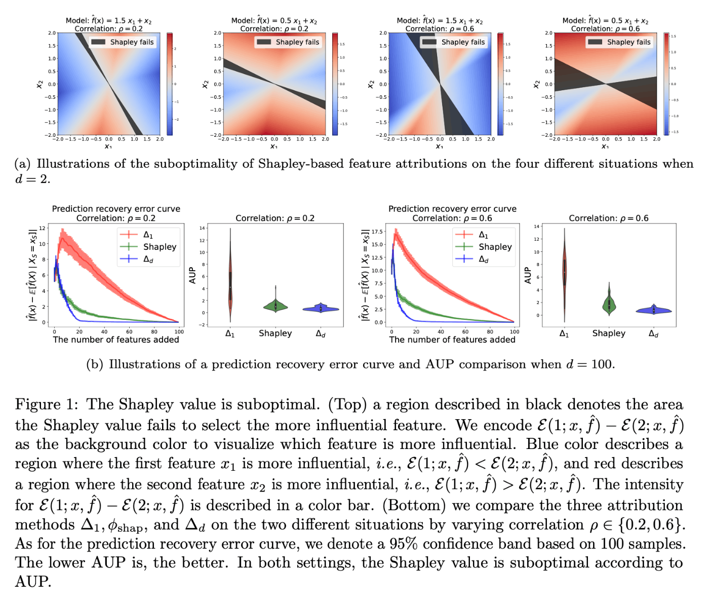
どのシーンでも、Shapley値がより影響力のある特徴を選択できない無視できない黒い領域が存在する。

WeightedSHAP

線形モデルを仮定した理論解析とシミュレーションの結果、特徴の相関が高い場合にShapley値が影響力のある特徴を選択できないようなシーンが出てきて、説明性が低くなるという結果が示された。
これを改善するため、限界貢献度の推定誤差を検討することで、限界貢献の加重平均を行う。

推定誤差の分析

Shapley値を推定するにあたり推定誤差が生じるが、この数学的定義から考えると推定誤差は限界貢献の推定誤差から生じている。
限界貢献の推定誤差について考えると、これは $v^{(\text{cond})}$ を推定するアルゴリズムと、 $∆_{j}$ を近似するためのサンプリングに基づくアルゴリズムに従っている。

次の図は定理から導かれる限界貢献 $Δ_{j}$ と推定限界貢献 $\hat{Δ}_{j}$ の相対的な差を連携サイズ $j \in [d]$ の関数として示している。ここで最も情報量の多い限界寄与である $∆_{d}$ が、真の値からの相対差が最も大きくなっている。すなわち $∆_{d}$ はモデル予測を説明する最大のシグナルなのだが、同時に推定誤差の意味で最も不安定になる。
これにより、シグナルを維持しながら推定誤差を減らすため、限界寄与の加重平均を考えるモチベーションが生まれてくる。

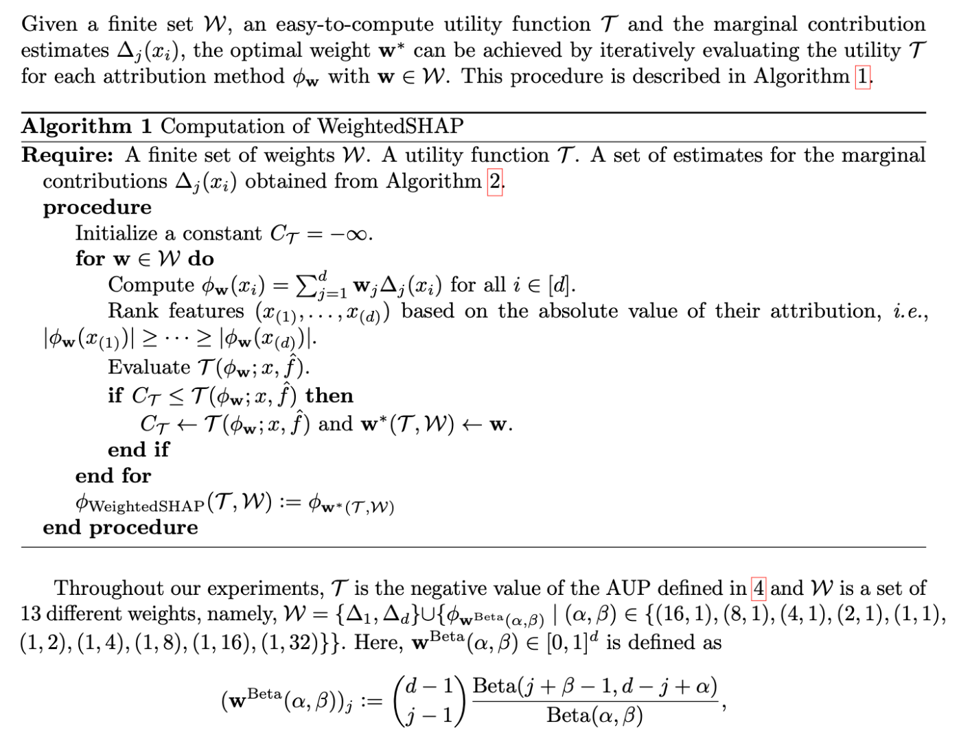
提案手法

φ_{\text{w}}(x_{i}) := \sum_{j=1}^{d} w_{j} Δ_{j}(x_{i})

これはゲーム理論において半価値の意味になっている式だが、効率公理(efficiency axiom)を満たす性質は帰属タスクではどうでもいい[4]ため、これを緩和することで一意性を犠牲に重み選択できるようにする。
この重み選択は下流タスクで選択することが望ましいらしいため、使用者が定義できるようにする。

重みの族 $\mathcal{W} ⊆ \{ w ∈ \mathbb{R}^d : \sum_{j=1}^{d} w_j = 1, w_j > 1 \}$
帰属法を入力とし、そのutilityを出力するユーザ定義の関数 $\mathcal{T}$
$\mathcal{T}$ は大きいほど良い (例えばnegative AUPなど)
$\bold{w}*(\mathcal{T},\mathcal{W}) := \text{argmax}_{w ∈ \mathcal{W}}\mathcal{T}( φ_{\bold{w}} )$

この設定によって、WeightedSHAPが提案される。

φ_{\text{WeightedSHAP}}(\mathcal{T},\mathcal{W}) := φ_{\bold{w}*(\mathcal{T},\mathcal{W})}

$W$ が一様分布を含む時、utility $\mathcal{T}$ に応じてWeightedSHAPはSHAPと同等か良いことが保証される。また $\mathcal{W}$ に含まれる重みベクトルが多いほどWeightedSHAP値の品質が向上する。

例えば negative AUPを $\mathcal{T}$ として、 $\{ Δ_{d}, φ_{\text{shap}} \} ⊆ \mathcal{W}$ のように使うと、WeightedSHAPは $Δ_{d}, φ_{\text{shap}}$ 両方より低いAUPを達成する。一様分布の重みは推定誤差を減らすかわりにシグナルを消失させてしまうが、WeightedSHAPは推定誤差を減らしながら、同時にシグナルを効率よく取っている。

[4] Mustapha Ridaoui, Michel Grabisch, and Christophe Labreuche. An axiomatisation of the banzhaf value and interaction index for multichoice games. In International Conference on Modeling Decisions for Artificial Intelligence, pages 143-155. Springer, 2018.

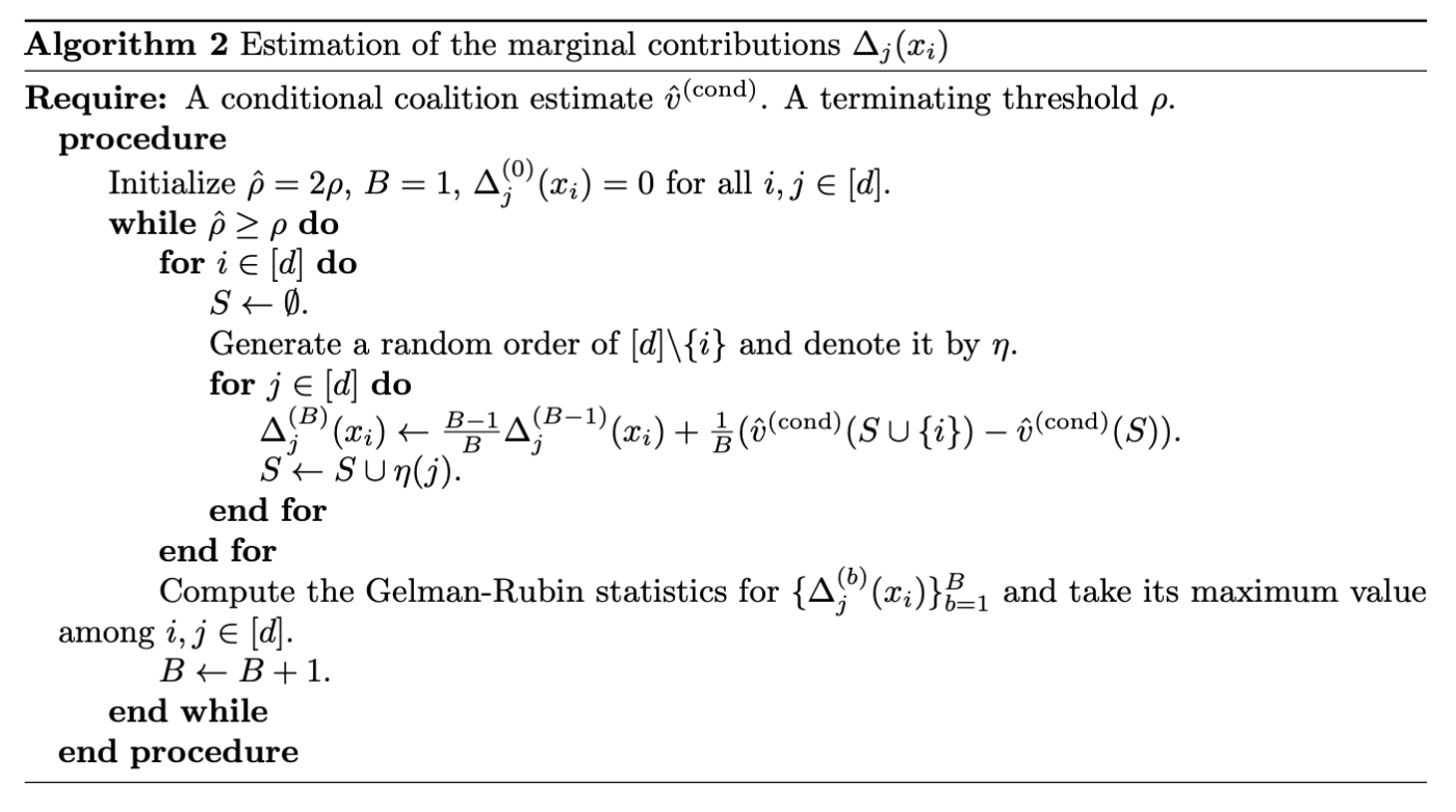
実装

$\mathcal{W}$ が有限集合で、 $\mathcal{T}$ が計算可能なutility関数であれば、最適な重み $w*$ は、各帰属法 $φ_{w}$ のutility $\mathcal{T}$ を $w ∈ \mathcal{W}$ で繰り返し評価することで計算できる。

重要な部分は、限界貢献の集合を推定すること、つまり $v^{(\text{cond})}$ の推定と $Δ_j$ の近似である。

まず $v^{(\text{cond})}$ の推定に関して、[5] [6] を参照すれば、入力特徴量の部分集合を入力に、同じ部分集合が与えられたときの予測値の条件付き期待値を出力する代理モデルを訓練する。この代理モデルはいい感じな条件で、特徴量の部分集合が与えられたときの予測値の条件付き期待値を、不偏推定できる。

$Δ_j$ の近似では、[7] [8]を参照すれば、加重平均をサンプリングベースのアルゴリズムで近似できる。疑似コードは次の画像のようになる。

[5] Christopher Frye, Damien de Mijolla, Tom Begley, Laurence Cowton, Megan Stanley, and Ilya Feige. Shapley explainability on the data manifold. arXiv preprint arXiv:2006.01272, 2020.

[6] Neil Jethani, Mukund Sudarshan, Ian Covert, Su-In Lee, and Rajesh Ranganath. Fastshap: Real-time shapley value estimation. arXiv preprint arXiv:2107.07436, 2021a.

[7] Amirata Ghorbani and James Zou. Data shapley: Equitable valuation of data for machine learning. In International Conference on Machine Learning, pages 2242-2251. PMLR, 2019.

[8] Yongchan Kwon and James Zou. Beta shapley: a unified and noise-reduced data valuation framework for machine learning. arXiv preprint arXiv:2110.14049, 2021.

実際のコードを眺めてみる。見やすさのため適宜改行などの改変をした。

Compute WeightedSHAP

weightedSHAP.generate_coalition_function creates a conditional coalition function that computes conditional expectation values $\mathbb{E} [f(X) \mid X_S = x_S]$

weightedSHAP.compute_attributions computes WeightedSHAP

$>\phi_{\mathrm{WeightedSHAP}}(\mathcal{T}, \mathcal{W}) := \phi_{\mathbf{w}^* (\mathcal{T}, \mathcal{W})}, >$
where $\mathbf{w}^* (\mathcal{T}, \mathcal{W}) := \mathrm{argmax}_{\mathbf{w} \in \mathcal{W}} \mathcal{T} (\phi_{\mathbf{w}})$ . By default, a set $\mathcal{W}$ includes SHAP and $\mathcal{T}$ is the negative area under the prediction recovery error curve (AUP, Equation (4) of the paper).

Example_fraud_inclusion_AUC.ipynb

problem = 'classification' 
dataset = 'fraud'
ML_model = 'boosting'

# train a baseline model
model_to_explain = weightedSHAP.create_model_to_explain(
    X_train, y_train, 
    X_val, y_val, 
    problem, 
    ML_model
    )

# Generate a conditional coalition function
conditional_extension = weightedSHAP.generate_coalition_function(
    model_to_explain, 
    X_train, X_est, 
    problem, 
    ML_model
    )
    
# With the conditional coalition function, we compute attributions
exp_dict = weightedSHAP.compute_attributions(
    problem, 
    ML_model,
    model_to_explain, conditional_extension,
    X_train, y_train,
    X_val, y_val, 
    X_test, y_test)

Analysis on WeightedSHAP

The output of weightedSHAP.compute_attributions includes

value_list: A list of WeightedSHAP values
true_list: A list of true labels
pred_list: A list of predictions
input_list: A list of inputs
cond_pred_keep_absolute: Conditional expectation of predictions. Features with large absolute values are added first.

Example_fraud_inclusion_AUC.ipynb

exp_dict.keys()
# -> ['value_list', 'true_list', 'pred_list', 'input_list', 'cond_pred_keep_absolute']

y_test=np.array(exp_dict['true_list'])
pred_list=np.array(exp_dict['pred_list'])
print(f'MSE of the original model: {np.mean((y_test-pred_list)**2):.3f}') 
# -> MSE of the original model: 0.226

最も興味のある部分として計算部分のメソッドを見てみる。外部のモジュールはすべて展開して書いた。

計算部分

weightedSHAPEngine.py

import tqdm
import numpy as np



def check_convergence(mem, n_require=100):
    """
    Compute Gelman-Rubin statistic
    Ref. https://arxiv.org/pdf/1812.09384.pdf (p.7, Eq.4)
    """
    if len(mem) < n_require:
        return 100
    n_chains=10
    (N, n_to_be_valued) = mem.shape

    if (N % n_chains) == 0:
        n_MC_sample = N//n_chains
        offset = 0
    else:
        n_MC_sample = N//n_chains
        offset = (N % n_chains)
    mem = mem[offset:]
    percent = 25
    
    while True:
        IQR_contstant = np.percentile(mem.reshape(-1), 50+percent) - np.percentile(mem.reshape(-1), 50-percent)
        if IQR_contstant == 0:
            percent = (50+percent)//2
            if percent >= 49:
                assert False, 'CHECK!!! IQR is zero!!!'
        else:
            break

    mem_tmp = mem.reshape(n_chains, n_MC_sample, n_to_be_valued)
    GR_list = []

    for j in range(n_to_be_valued):
        mem_tmp_j_original = mem_tmp[:,:,j].T # now we have (n_MC_sample, n_chains)
        mem_tmp_j = mem_tmp_j_original/IQR_contstant
        mem_tmp_j_mean = np.mean(mem_tmp_j, axis=0)
        s_term = np.sum((mem_tmp_j-mem_tmp_j_mean)**2)/(n_chains*(n_MC_sample-1)) # + 1e-16 this could lead to wrong estimator
        if s_term == 0:
            continue

        mu_hat_j = np.mean(mem_tmp_j)
        B_term = n_MC_sample*np.sum((mem_tmp_j_mean-mu_hat_j)**2)/(n_chains-1)
        GR_stat = np.sqrt((n_MC_sample-1)/n_MC_sample + B_term/(s_term*n_MC_sample))
        GR_list.append(GR_stat)

    GR_stat = np.max(GR_list)
    print(f'Total number of random sets: {len(mem)}, GR_stat: {GR_stat}', flush=True)
    return GR_stat 



def compute_predict(model_to_explain, x, problem, ML_model):
    if (ML_model == 'linear') and (problem == 'classification'):
        return float(model_to_explain.predict_proba(x)[:,1])
    else:
        return float(model_to_explain.predict(x))



def beta_constant(a, b):
    """
    the second argument (b; beta) should be integer in this function
    """
    beta_fct_value = 1/a
    for i in range(1,b):
        beta_fct_value = beta_fct_value*(i/(a+i))
    return beta_fct_value
    


def compute_weight_list(m, alpha=1, beta=1):
    """
    Given a prior distribution (beta distribution (alpha,beta))
    beta_constant(j+1, m-j) = j! (m-j-1)! / (m-1)! / m # which is exactly the Shapley weights.

    # weight_list[n] is a weight when baseline model uses 'n' samples (w^{(n)}(j)*binom{n-1}{j} in the paper).
    """
    weight_list=np.zeros(m)
    normalizing_constant=1/beta_constant(alpha, beta)
    for j in np.arange(m):
        # when the cardinality of random sets is j
        weight_list[j]=beta_constant(j+alpha, m-j+beta-1)/beta_constant(j+1, m-j)
        weight_list[j]=normalizing_constant*weight_list[j] # we need this '/m' but omit for stability # normalizing
    return weight_list/np.sum(weight_list)



def compute_semivalue_from_MC(marginal_contrib, semivalue_list):
    """
    With the marginal contribution values, it computes semivalues
    """
    semivalue_dict = {}
    n_elements=marginal_contrib.shape[0]
    for weight in semivalue_list:
        alpha, beta=weight
        if alpha > 0:
            model_name=f'Beta({beta},{alpha})'
            weight_list = compute_weight_list(m=n_elements, alpha=alpha, beta=beta)
        else:
            if beta == 'LOO-First':
                model_name = 'LOO-First'
                weight_list = np.zeros(n_elements) 
                weight_list[0] = 1
            elif beta == 'LOO-Last':
                model_name = 'LOO-Last'
                weight_list = np.zeros(n_elements) 
                weight_list[-1] = 1
        
        if len(marginal_contrib.shape) == 2:
            semivalue_tmp = np.einsum('ij,j->i', marginal_contrib, weight_list)
        else:
            # classification case
            semivalue_tmp = np.einsum('ijk,j->ik', marginal_contrib, weight_list)
        semivalue_dict[model_name] = semivalue_tmp
    return semivalue_dict



def compute_cond_pred_list(attribution_dict, game, more_important_first=True):
    n_features = game.players
    n_max_features = n_features  # min(n_features, 200)

    cond_pred_list = []
    for method in attribution_dict.keys():
        cond_pred_list_tmp = []
        if more_important_first is True:
            # more important to less important (large to zero)
            sorted_index = np.argsort(np.abs(attribution_dict[method]))[::-1]
        else:
            # less important to more important (zero to large)
            sorted_index = np.argsort(np.abs(attribution_dict[method]))
        
        for n_top in range(n_max_features+1):
            top_index = sorted_index[:n_top]
            S = np.zeros(n_features, dtype=bool)
            S[top_index] = True
            
            # prediction recovery error
            cond_pred_list_tmp.append(game(S)) 
        cond_pred_list.append(cond_pred_list_tmp)

    return cond_pred_list



class PredictionGame:
    """
    Cooperative game for an individual example's prediction.
    Reference: https://github.com/iancovert/removal-explanations/blob/main/rexplain/behavior.py

    Args:
      extension: model extension (see removal.py).
      sample: numpy array representing a single model input.
    """

    def __init__(self, extension, sample, superpixel_size=1):
        # Add batch dimension to sample.
        if sample.ndim == 1:
            sample = sample[np.newaxis]
        # elif sample.shape[0] != 1:
        # raise ValueError('sample must have shape (ndim,) or (1,ndim)')

        self.extension = extension
        self.sample = sample
        self.players = np.prod(sample.shape)//(superpixel_size**2)//sample.shape[0] # sample.shape[1]

        # Caching.
        self.sample_repeat = sample

    def __call__(self, S):
        # Return scalar if single subset.
        single_eval = (S.ndim == 1)
        if single_eval:
            S = S[np.newaxis]
            input_data = self.sample
        else:
            # Try to use caching for repeated data.
            if len(S) != len(self.sample_repeat):
                self.sample_repeat = self.sample.repeat(len(S), 0)
            input_data = self.sample_repeat

        # Evaluate.
        output = self.extension(input_data, S)
        if single_eval:
            output = output[0]
        return output



semivalue_list = [
    (-1,'LOO-First'), (1,32), (1,16), (1, 8), (1, 4), (1, 2), 
    (1,1), (2,1), (4,1), (8, 1), (16, 1), (32,1), (-1,'LOO-Last')
    ]
attribution_list = [
    'LOO-First', 'Beta(32,1)', 'Beta(16,1)', 'Beta(8,1)', 
    'Beta(4,1)', 'Beta(2,1)', 'Beta(1,1)', 'Beta(1,2)',
    'Beta(1,4)', 'Beta(1,8)', 'Beta(1,16)', 'Beta(1,32)', 'LOO-Last'
    ]



def MarginalContributionValue(
        game, 
        thresh=1.005, 
        batch_size=1, 
        n_check_period=100
        ):
    """
    Calculate feature attributions using the marginal contributions.
    """

    # index of the added feature, cardinality of set
    arange = np.arange(batch_size)
    output = game(np.zeros(game.players, dtype=bool))
    MC_size = [game.players, game.players] + list(output.shape)
    MC_mat = np.zeros(MC_size) 
    MC_count = np.zeros((game.players, game.players))

    converged = False
    n_iter = 0
    marginal_contribs = np.zeros([0, np.prod([game.players] + list(output.shape))]) 

    while not converged:
        for _ in range(n_check_period):

            # Sample permutations.
            permutations = np.tile(np.arange(game.players), (batch_size, 1))
            for row in permutations:
                np.random.shuffle(row)
            S = np.zeros((batch_size, game.players), dtype=bool)

            # Unroll permutations.
            prev_value = game(S)
            marginal_contribs_tmp = np.zeros(([batch_size, game.players] + list(output.shape)))
            for j in range(game.players):
                """
                Marginal contribution estimates with respect to j samples
                j = 0 means LOO-First
                """
                S[arange, permutations[:, j]] = 1
                next_value = game(S)
                MC_mat[permutations[:, j], j] += (next_value - prev_value)
                MC_count[permutations[:, j], j] += 1
                marginal_contribs_tmp[arange, permutations[:, j]] = (next_value - prev_value)

                # update
                prev_value = next_value
            marginal_contribs = np.concatenate([marginal_contribs, marginal_contribs_tmp.reshape(batch_size,-1)], axis=0)
            
        if (n_iter+1) == 100:
            converged=True
        elif (n_iter+1) >= 2:
            if check_convergence(marginal_contribs) < thresh: 
                print(f'Therehosld: {int(0.999*(game.players*n_check_period))}')
                converged = True
        else:
            pass

        n_iter += 1

    print(f'We have seen {((n_iter+1)*n_check_period*batch_size)} random subsets for each feature.')
    if len(MC_mat.shape) != 2:
        # classification case
        MC_count = np.repeat(MC_count, MC_mat.shape[-1], axis=-1).reshape(MC_mat.shape)
    
    return MC_mat, MC_count



def compute_attributions(
    problem, 
    ML_model, 
    model_to_explain, 
    conditional_extension, 
    X_test, y_test, 
    n_max=100
    ):
    """
    Compute attribution values and evaluate its performance
    """

    pred_list, pred_masking = [], []
    cond_pred_keep_absolute, cond_pred_remove_absolute=[], []
    value_list = []
    n_max = min(n_max, len(X_test))

    for ind in tqdm.tqdm(range(n_max)):

        # Store original prediction 
        original_pred = compute_predict(model_to_explain, X_test[ind,:].reshape(1,-1), problem, ML_model)
        pred_list.append(original_pred)

        # Estimate marginal contributions
        conditional_game = PredictionGame(conditional_extension, X_test[ind, :])
        MC_conditional_mat, MC_conditional_count = MarginalContributionValue(conditional_game) 
        MC_est = np.array(MC_conditional_mat/(MC_conditional_count+1e-16))
        
        # Optimize weight for WeightedSHAP (By default, AUP is used)
        attribution_dict_all = compute_semivalue_from_MC(MC_est, semivalue_list)
        cond_pred_keep_absolute_list = compute_cond_pred_list(attribution_dict_all, conditional_game)
        AUP_list = np.sum(np.abs(np.array(cond_pred_keep_absolute_list)- original_pred), axis=1)
        WeightedSHAP_index = np.argmin(AUP_list)
        value_list.append(attribution_dict_all[attribution_list[WeightedSHAP_index]])

        """
        Evaluation
        """
        # Conditional prediction from most important to least important (keep absolte)
        cond_pred_keep_absolute_list = compute_cond_pred_list(attribution_dict_all, conditional_game)
        cond_pred_keep_absolute.append(cond_pred_keep_absolute_list)

    exp_dict=dict()
    exp_dict['value_list'] = value_list
    exp_dict['true_list'] = np.array(y_test)[:n_max]
    exp_dict['pred_list'] = np.array(pred_list)  
    exp_dict['input_list'] = np.array(X_test)[:n_max]  
    exp_dict['cond_pred_keep_absolute'] = np.array(cond_pred_keep_absolute)   

    return exp_dict

実験結果

marginal contribution feature importance (MCI) や予測回復誤差タスク、包含性能タスクにおけるShapley値と比較し、与えられた特徴量の数でモデルの予測値がどれだけ回復するかを測定することで、帰属の良さを評価する。
モデルの性能については、回帰問題ではMSE、分類問題ではAUCを評価する。

$v^{(\text{cond})}$ の代理モデルとして2層のMLPを使う。
$\mathcal{T}$ はnegative AUP
$\mathcal{W}$ は $Δ_1, Δ_d, φ_{\text{shap}}$ を含む13種類の重み集合

この設定でWeightedSHAP(赤)、 MCI(青)、Shapley値(緑)の予測回復誤差曲線をプロットしたものが次の図である。

また、画像タスクにおいてCNNの評価を行った。

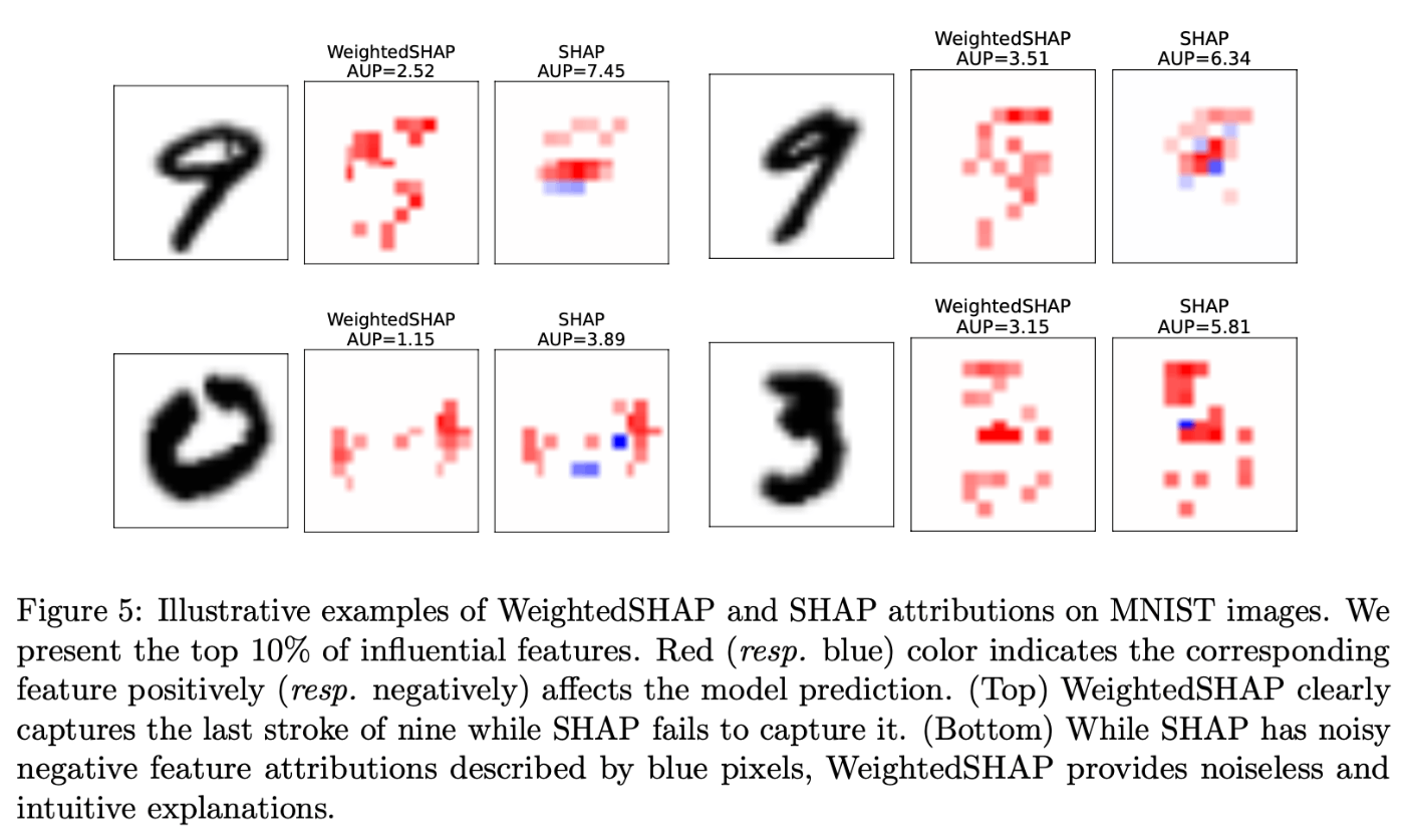
課題

元論文ではAUPを評価指標として使用し重みを最適化したが、特徴帰属法を評価するための統一的な指標は無いので、異分野にいる人は帰属概念を気にするかもしれない。したがって用途に最適化された限界貢献重み付けのバリエーションを開発することが今後の方向性としてある。

また、今回SHAPとWeightedSHAPを比較したが、[9] [10] はSHAPと他の評価指標を比較している。これは元論文を補完した研究になっている。

[9] Chih-Kuan Yeh, Cheng-Yu Hsieh, Arun Suggala, David I Inouye, and Pradeep K Ravikumar. On the (in) fidelity and sensitivity of explanations. Advances in Neural Information Processing Systems, 32, 2019.

[10] Neil Jethani, Mukund Sudarshan, Ian Covert, Su-In Lee, and Rajesh Ranganath. Fastshap: Real-time shapley value estimation. arXiv preprint arXiv:2107.07436, 2021a.

感想

SHAPは表データのみでなく、言語トークンを用いたモデルや画像などでも使えて、モデルを変更するのではなく特徴量のバリエーションから比較することができる。
WeightedSHAPを使えばSHAPよりも良い貢献度分解が可能になるため、使い得だと思った。