"EfficientViT" by MIT and MSResearch 実装と解説
[1] Han Cai, Junyan Li, Muyan Hu, Chuang Gan, Song Han
"EfficientViT: Multi-Scale Linear Attention for High-Resolution Dense Prediction"
2022-05-29, ICCV 2023
https://arxiv.org/abs/2205.14756
[2] Xinyu Liu, Houwen Peng, Ningxin Zheng, Yuqing Yang, Han Hu, Yixuan Yuan
"EfficientViT: Memory Efficient Vision Transformer with Cascaded Group Attention"
Proceedings of the IEEE/CVF Conference on Computer Vision and Pattern Recognition
2023-05-11, CVPR 2023
https://arxiv.org/abs/2305.07027
MITのEfficientViTとMSResearch(Asia)のEfficientViTを比較しながら実装します。
論文を斜め読みして、作ってみた所感としては以下のように思いました。
- MITのEfficientViTはどちらかというとEfficient CoAtNetで、現実的な精度が出る。EfficientNetv2より高効率。
- MSResearchのEfficientViTは、ViTというよりもAttentionを使ったMobileNet。ONNXなどの現実的な実装まで速度を測定している点は良い。
どちらも良い研究だが、個人的には「Efficient"ViT"」というにはCNN過ぎたり構造が複雑すぎたりしてると思う。(EfficientFormerも殆どCoAtNetなので、ViT自体が非効率だというコモンセンスができてるのかもしれないが...)
使用感の比較
ImageNet上での精度
timmのベンチマークは以下のテーブル。efficientvit_bがMIT、efficientvit_mがMSResearchのモデル。
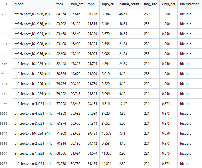
公称値の精度で言えばMITの方が良い。
速度
精度以外の部分について、MITとMSResearchでどのような違いがあるか、次の項目について測ってみた。
- 単位枚数あたりの推論時間(throughput)
- パラメータ数
- 和積演算回数(MACs)
throughputについては、[32, 3, 224, 224] の入力を複数回行い、平均タイムを計測した。パラメータ数とMACsについてはtorchinfoの計算を借りた。
以下計測結果。環境はtorch2.1.1, timm0.9.12, CPU i7-9700, GPU Quadro P5000, CUDA 12.2, CUDNN 8。
cpu          /sec   acc      prams   GMACs
effvit mit1: 0.712  79.252    9.10   0.5121
effvit msr5: 0.260  77.058   12.47   0.5165
effnetv2 b0: 0.605  78.358    7.14   0.7181
effnetv2 b2: 0.818  80.196   10.10(260px)

gpu
effvit mit1: 0.056
effvit msr5: 0.048
effnetv2 b0: 0.052
effnetv2 b2: 0.069
参考としてEfficientNet b0 b2も計測した。ImageNetベンチマークの精度はtimmの測定に基づく。(EfficientNet-b2は入力空間方向もスケールしているので単純比較はできない点に注意)
結果から分かる通り、MSResearchの方は精度は2%程度低いもののcpu推論のthroughputが桁違いに速い。同時に、論文でよく示されているFLOPsやパラメータ数の比較がいかにあてにならないかも良く表している。
以上の計測で得られたモチベーションから、この秘密を論文と実装から解き明かしてみる。
EfficientViT by MIT
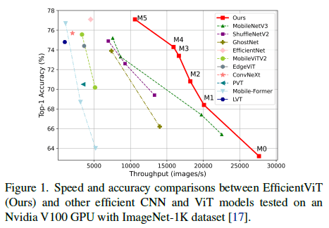
MITのEfficientViTは、主にSegmentationなどの「高解像度の密な予測」を高効率に計算することを念頭に設計された。SoftMax Attentionや大きなConv kernelなどを効率化し、Multi-Scale Linear Attentionに変えることで、受容野の広さやマルチスケール学習に有利な高効率ViTを作ることができたらしい。
 [1]より、他モデルとの速度比較
MITのモデルは、EfiicientNetのMBConvを最初の層で行い(CoAtNetやCAFormerっぽい)、Linear Attentionを計算するKeyとValを事前に畳み込みで小さくして計算コストを抑えている。
CityScapeとADE20kのようなタスクのセグメンテーションモデルにおいて、SegNeXtなどと比較して高い精度効率を示していて、ImageNetでは巨大GPUでは微妙な差にとどまっているが、Jetsonのような比較的低性能なエッジデバイスでは目に見えて良い速度性能を示している。
ReLU Linear Attention
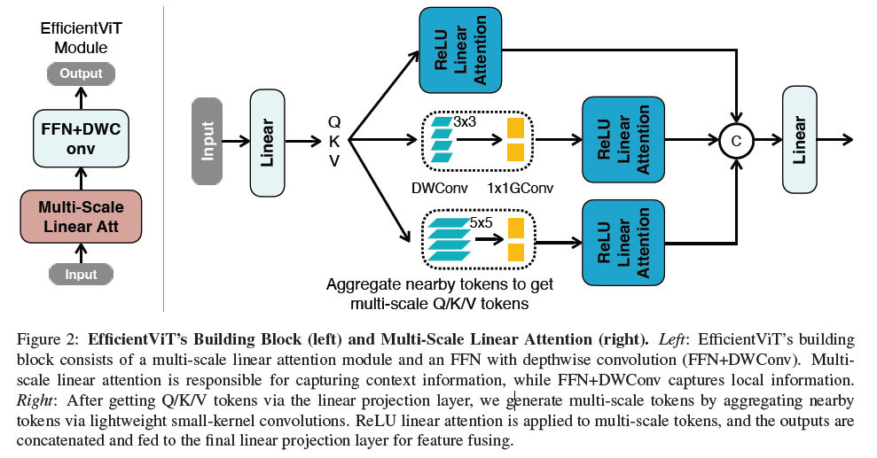 [1]より、EfficientViT Blockの設計
単純なViTBlock(fully featured Transformer)との違いは以下。
- 内積を使うAttentionのかわりにLinear Attentionを使う
- 類似度計算にSoftMaxではなくReLUを使う
Linear Attentionは[3]で有名なもので、以下の図がわかりやすい。
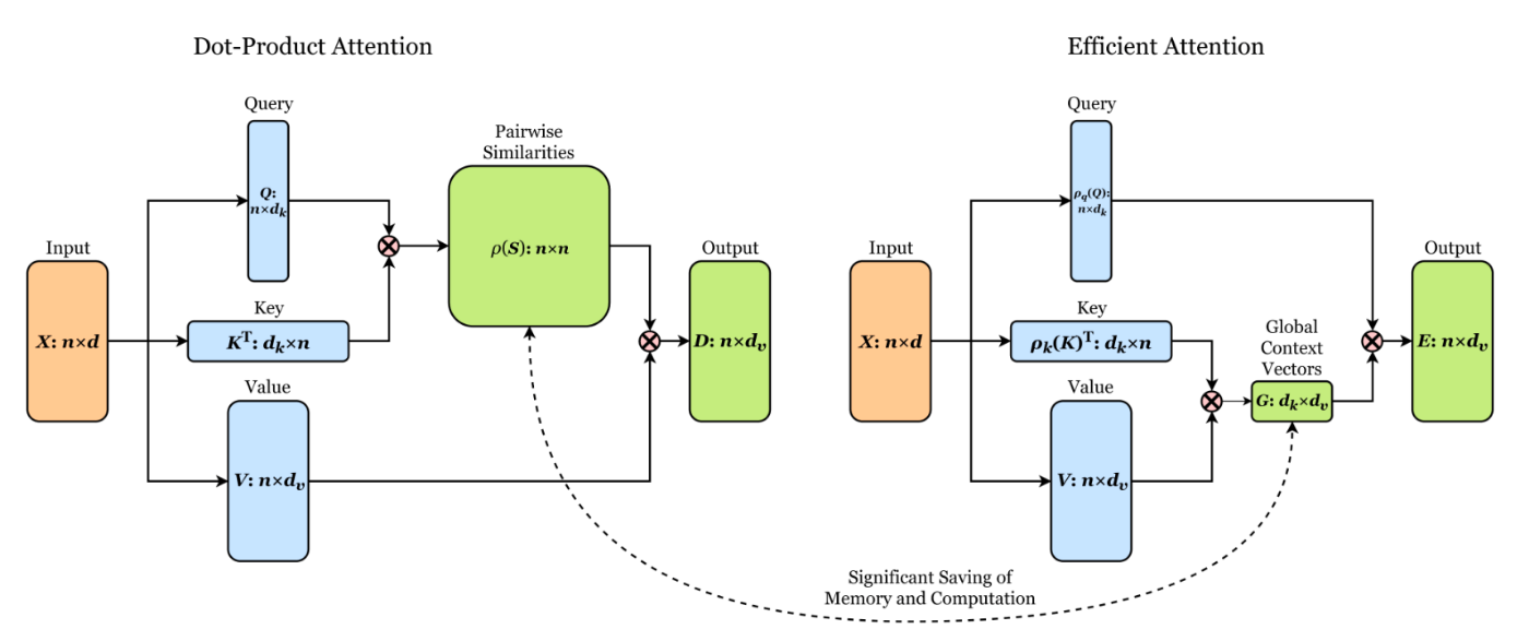 [4]より、通常のAttentionとLinear Attentionの比較図
[3] Angelos Katharopoulos, Apoorv Vyas, Nikolaos Pappas, François Fleuret
"Transformers are RNNs: Fast Autoregressive Transformers with Linear Attention"
Proceedings of the International Conference on Machine Learning (ICML) 2022
[4] lucidrains
"Linear Attention Transformer"
https://github.com/lucidrains/linear-attention-transformer
すなわち、
このLinear Attentionの類似度計算部分にReLUを用いたのがMITのEffficientViT Blockで、以下の式の
通常のAttentionは
しかし、ReLUは非線形類似関数を持たない(?)ので、シャープなAttentionを作れない、つまり局所情報抽出能力はSoftMaxよりも弱いという欠点もある。
 [1]より、Attentionの違いと可視化
モデルのスケーリング
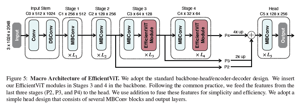 [1]より、EfficientViTのアーキテクチャ
timmの実装で、最も小さいEfficientViT-b1を見てみる。入力は256×256pxの画像。
===========================================================================================
Layer (type (var_name))                  Input Shape               Output Shape
===========================================================================================
EfficientVit (EfficientVit)                 [1, 3, 256, 256]          [1, 1000]
├─Stem (stem)                               [1, 3, 256, 256]          [1, 16, 128, 128]
│    └─ConvNormAct (in_conv)                [1, 3, 256, 256]          [1, 16, 128, 128]
│    └─ResidualBlock (res0)                 [1, 16, 128, 128]         [1, 16, 128, 128]
├─Sequential (stages)                       [1, 16, 128, 128]         [1, 256, 8, 8]
│    └─EfficientVitStage (0)                [1, 16, 128, 128]         [1, 32, 64, 64]
│    │    └─ResidualBlock (0)               [1, 16, 128, 128]         [1, 32, 64, 64]
│    │    └─ResidualBlock (1)               [1, 32, 64, 64]           [1, 32, 64, 64]
│    └─EfficientVitStage (1)                [1, 32, 64, 64]           [1, 64, 32, 32]
│    │    └─ResidualBlock (0)               [1, 32, 64, 64]           [1, 64, 32, 32]
│    │    └─ResidualBlock (1)               [1, 64, 32, 32]           [1, 64, 32, 32]
│    │    └─ResidualBlock (2)               [1, 64, 32, 32]           [1, 64, 32, 32]
│    └─EfficientVitStage (2)                [1, 64, 32, 32]           [1, 128, 16, 16]
│    │    └─ResidualBlock (0)               [1, 64, 32, 32]           [1, 128, 16, 16]
│    │    └─EfficientVitBlock (1)           [1, 128, 16, 16]          [1, 128, 16, 16]
│    │    └─EfficientVitBlock (2)           [1, 128, 16, 16]          [1, 128, 16, 16]
│    │    └─EfficientVitBlock (3)           [1, 128, 16, 16]          [1, 128, 16, 16]
│    └─EfficientVitStage (3)                [1, 128, 16, 16]          [1, 256, 8, 8]
│    │    └─ResidualBlock (0)               [1, 128, 16, 16]          [1, 256, 8, 8]
│    │    └─EfficientVitBlock (1)           [1, 256, 8, 8]            [1, 256, 8, 8]
│    │    └─EfficientVitBlock (2)           [1, 256, 8, 8]            [1, 256, 8, 8]
│    │    └─EfficientVitBlock (3)           [1, 256, 8, 8]            [1, 256, 8, 8]
│    │    └─EfficientVitBlock (4)           [1, 256, 8, 8]            [1, 256, 8, 8]
├─ClassifierHead (head)                     [1, 256, 8, 8]            [1, 1000]
│    └─ConvNormAct (in_conv)                [1, 256, 8, 8]            [1, 1536, 8, 8]
│    └─SelectAdaptivePool2d (global_pool)   [1, 1536, 8, 8]           [1, 1536]
│    │    └─AdaptiveAvgPool2d (pool)        [1, 1536, 8, 8]           [1, 1536, 1, 1]
│    │    └─Flatten (flatten)               [1, 1536, 1, 1]           [1, 1536]
│    └─Sequential (classifier)              [1, 1536]                 [1, 1000]
これを各モデルスケールで見て、図上のLについて以下にまとめた。
| L1 | L2 | L3 | L4 | |
|---|---|---|---|---|
| b1 | 2 | 3 | 3 | 4 |
| b2 | 3 | 4 | 4 | 6 |
| b3 | 4 | 6 | 6 | 9 |
Transformer系だと[
性能評価
図に並んでいるモデルでは(当然ながら)最高の性能が出ている。
 [1]より、ImageNetにおける評価
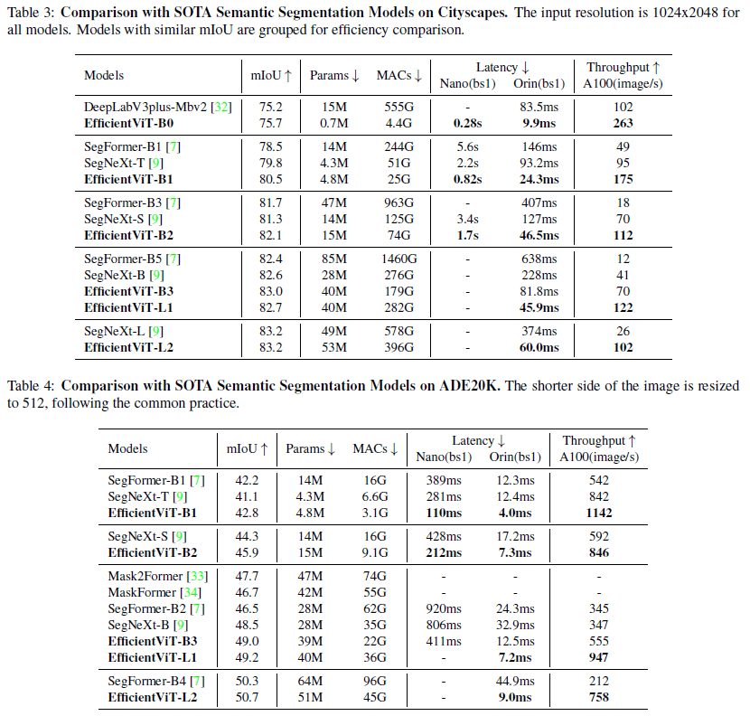 [1]より、Segmentationタスクの評価
timmのモデルで比較してみると、EfficientViT-b1はResNet-RS 50と同精度でMACsは1/10、枝刈りを行ったEfficientNet-b2と殆ど同じ精度とMACsとなっている。b1でもある程度の性能が保証されているようだ。
一般のご家庭にあるGPUでは大体b1,b2スケールで使用できる雰囲気に感じた。
EffficientViT by MSResearch
MSResearchのEfficientViTは、Segmentationの特徴抽出部分を置き換えるMITのものとは異なり、MobileNet系の位置と競合している。
 [2]より、速度精度の比較
解析
前述の通り、FLOPsに関しての解析は多いがこれは正確な速度の指標ではない。論文中ではGPU V100上でMobileViT-XS(700MFLOPs)よりもDeiT-T(1220MFLOPs)のほうが速く、MobileViT系の手法はDeiTやSwinより深掘りされていないことが挙げられていて、これは経験的にも正しい感じがある。
[5]でも述べられていたが、推論や学習の演算グラフそのものよりも、メモリアクセスが速度に悪さするという事実があり、ViTにおいては特にMulti-Head Attention(MA)のReshapeがメモリアクセスを占有していて、さらに要素ごとの関数もよくないらしい。
MSResearchはメモリアクセスを解析し、MAとFFNの層の比率を最適にすることで、性能を損なわずメモリ効率も良くできることを示した。層が多いとAttentionのいくつかは線形な処理を学習してしまい、冗長になってしまう。MSResearchのEfficientViTは既存の[
つまり、Attentionをどうこうするのではなく、効率のいいAttentionとFFNのブロック配置を作るというのが要旨である。
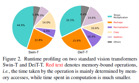 [2]より、メモリアクセス時間の占有率
[5] Weihao Yu, Pan Zhou, Shuicheng Yan, Xinchao Wang
"InceptionNeXt: When Inception Meets ConvNeXt"
https://arxiv.org/abs/2303.16900
https://github.com/sail-sg/inceptionnext
Swin-TとDeiT-Tのスケーリングを弄り、Attentionの利用率を適切に下げることでメモリ効率性を高めることができる。(性能を向上と書かれているが、あまり向上しているようには見えない...)
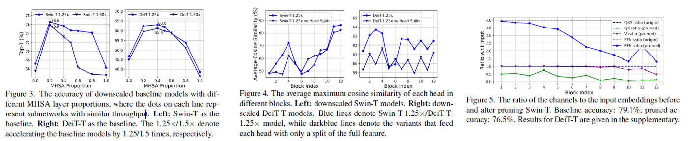 [2]より、SwinとDeiTのレイヤーをダウンスケールしたときの精度、各Attetnion出力の類似度(つまり高い場合は似た特徴を学習している)、枝刈り時のAttentionの埋め込みのチャンネル比率(?)
モデル設計
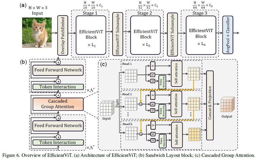 [2]より、モデルのアーキテクチャとCascaded Group Attention
MSResearchのモデルは魔改造されていて少し複雑になっている。
まず、通常のスケーリングではなく、3ステージ構成になっている。そして通常のAttention Norm FFN Normの部分がToken Interaction(Conv Norm×1)とFFN(Conv Norm Act Conv Norm)とCascaded Group Attentionのサンドウィッチになっている。
例えば、timmのEfficientViT-m5は以下のようになっている。
EfficientViT-m5
======================================================================================================
Layer (type (var_name))                                 Input Shape               Output Shape
======================================================================================================
EfficientVitMsra (EfficientVitMsra)                    [1, 3, 224, 224]          [1, 1000]
├─PatchEmbedding (patch_embed)                         [1, 3, 224, 224]          [1, 192, 14, 14]
│    └─ConvNorm (conv1)                                [1, 3, 224, 224]          [1, 24, 112, 112]
│    └─ReLU (relu1)                                    [1, 24, 112, 112]         [1, 24, 112, 112]
│    └─ConvNorm (conv2)                                [1, 24, 112, 112]         [1, 48, 56, 56]
│    └─ReLU (relu2)                                    [1, 48, 56, 56]           [1, 48, 56, 56]
│    └─ConvNorm (conv3)                                [1, 48, 56, 56]           [1, 96, 28, 28]
│    └─ReLU (relu3)                                    [1, 96, 28, 28]           [1, 96, 28, 28]
│    └─ConvNorm (conv4)                                [1, 96, 28, 28]           [1, 192, 14, 14]
├─Sequential (stages)                                  [1, 192, 14, 14]          [1, 384, 4, 4]
│    └─EfficientVitStage (0)                           [1, 192, 14, 14]          [1, 192, 14, 14]
│    │    └─Sequential (blocks)                        [1, 192, 14, 14]          [1, 192, 14, 14]
│    │    │    └─EfficientVitBlock (0)                 [1, 192, 14, 14]          [1, 192, 14, 14]
│    │    │    │    └─ResidualDrop (dw0)               [1, 192, 14, 14]          [1, 192, 14, 14]
│    │    │    │    │    └─ConvNorm (m)                [1, 192, 14, 14]          [1, 192, 14, 14]
│    │    │    │    └─ResidualDrop (ffn0)              [1, 192, 14, 14]          [1, 192, 14, 14]
│    │    │    │    │    └─ConvMlp (m)                 [1, 192, 14, 14]          [1, 192, 14, 14]
│    │    │    │    └─ResidualDrop (mixer)             [1, 192, 14, 14]          [1, 192, 14, 14]
│    │    │    │    │    └─LocalWindowAttention (m)    [1, 192, 14, 14]          [1, 192, 14, 14]
│    │    │    │    │    │    └─CascadedGroupAttention [4, 192, 7, 7]            [4, 192, 7, 7]
│    │    │    │    │    │    │    └─ModuleList (qkvs) --                        --
│    │    │    │    │    │    │    └─ModuleList (dws)  --                        --
│    │    │    │    │    │    │    └─ModuleList (qkvs) --                        --
│    │    │    │    │    │    │    └─ModuleList (dws)  --                        --
│    │    │    │    │    │    │    └─ModuleList (qkvs) --                        --
│    │    │    │    │    │    │    └─ModuleList (dws)  --                        --
│    │    │    │    │    │    │    └─Sequential (proj) [4, 192, 7, 7]            [4, 192, 7, 7]
│    │    │    │    └─ResidualDrop (dw1)               [1, 192, 14, 14]          [1, 192, 14, 14]
│    │    │    │    │    └─ConvNorm (m)                [1, 192, 14, 14]          [1, 192, 14, 14]
│    │    │    │    └─ResidualDrop (ffn1)              [1, 192, 14, 14]          [1, 192, 14, 14]
│    │    │    │    │    └─ConvMlp (m)                 [1, 192, 14, 14]          [1, 192, 14, 14]
│    │    │    │    │    │    └─ConvNorm (pw1)         [1, 192, 14, 14]          [1, 384, 14, 14]
│    │    │    │    │    │    └─ReLU (act)             [1, 384, 14, 14]          [1, 384, 14, 14]
│    │    │    │    │    │    └─ConvNorm (pw2)         [1, 384, 14, 14]          [1, 192, 14, 14]
│    └─EfficientVitStage (1)                           [1, 192, 14, 14]          [1, 288, 7, 7]
│    │    └─Sequential (downsample)                    [1, 192, 14, 14]          [1, 288, 7, 7]
│    │    │    └─Sequential (res1)                     [1, 192, 14, 14]          [1, 192, 14, 14]
│    │    │    │    └─ResidualDrop (0)                 [1, 192, 14, 14]          [1, 192, 14, 14]
│    │    │    │    │    └─ConvNorm (m)                [1, 192, 14, 14]          [1, 192, 14, 14]
│    │    │    │    └─ResidualDrop (1)                 [1, 192, 14, 14]          [1, 192, 14, 14]
│    │    │    │    │    └─ConvMlp (m)                 [1, 192, 14, 14]          [1, 192, 14, 14]
│    │    │    └─PatchMerging (patchmerge)             [1, 192, 14, 14]          [1, 288, 7, 7]
│    │    │    │    └─ConvNorm (conv1)                 [1, 192, 14, 14]          [1, 768, 14, 14]
│    │    │    │    └─ReLU (act)                       [1, 768, 14, 14]          [1, 768, 14, 14]
│    │    │    │    └─ConvNorm (conv2)                 [1, 768, 14, 14]          [1, 768, 7, 7]
│    │    │    │    └─ReLU (act)                       [1, 768, 7, 7]            [1, 768, 7, 7]
│    │    │    │    └─SEModule (se)                    [1, 768, 7, 7]            [1, 768, 7, 7]
│    │    │    │    │    └─Conv2d (fc1)                [1, 768, 1, 1]            [1, 192, 1, 1]
│    │    │    │    │    └─Identity (bn)               [1, 192, 1, 1]            [1, 192, 1, 1]
│    │    │    │    │    └─ReLU (act)                  [1, 192, 1, 1]            [1, 192, 1, 1]
│    │    │    │    │    └─Conv2d (fc2)                [1, 192, 1, 1]            [1, 768, 1, 1]
│    │    │    │    │    └─Sigmoid (gate)              [1, 768, 1, 1]            [1, 768, 1, 1]
│    │    │    │    └─ConvNorm (conv3)                 [1, 768, 7, 7]            [1, 288, 7, 7]
│    │    │    └─Sequential (res2)                     [1, 288, 7, 7]            [1, 288, 7, 7]
│    │    │    │    └─ResidualDrop (0)                 [1, 288, 7, 7]            [1, 288, 7, 7]
│    │    │    │    │    └─ConvNorm (m)                [1, 288, 7, 7]            [1, 288, 7, 7]
│    │    │    │    └─ResidualDrop (1)                 [1, 288, 7, 7]            [1, 288, 7, 7]
│    │    │    │    │    └─ConvMlp (m)                 [1, 288, 7, 7]            [1, 288, 7, 7]
│    │    └─Sequential (blocks)                        [1, 288, 7, 7]            [1, 288, 7, 7]
│    │    │    └─EfficientVitBlock (0)                 [1, 288, 7, 7]            [1, 288, 7, 7]
│    │    │    └─EfficientVitBlock (1)                 [1, 288, 7, 7]            [1, 288, 7, 7]
│    │    │    └─EfficientVitBlock (2)                 [1, 288, 7, 7]            [1, 288, 7, 7]
│    └─EfficientVitStage (2)                           [1, 288, 7, 7]            [1, 384, 4, 4]
│    │    └─Sequential (downsample)                    [1, 288, 7, 7]            [1, 384, 4, 4]
│    │    └─Sequential (blocks)                        [1, 384, 4, 4]            [1, 384, 4, 4]
│    │    │    └─EfficientVitBlock (0)                 [1, 384, 4, 4]            [1, 384, 4, 4]
│    │    │    └─EfficientVitBlock (1)                 [1, 384, 4, 4]            [1, 384, 4, 4]
│    │    │    └─EfficientVitBlock (2)                 [1, 384, 4, 4]            [1, 384, 4, 4]
│    │    │    └─EfficientVitBlock (3)                 [1, 384, 4, 4]            [1, 384, 4, 4]
├─SelectAdaptivePool2d (global_pool)                   [1, 384, 4, 4]            [1, 384]
│    └─AdaptiveAvgPool2d (pool)                        [1, 384, 4, 4]            [1, 384, 1, 1]
│    └─Flatten (flatten)                               [1, 384, 1, 1]            [1, 384]
├─NormLinear (head)                                    [1, 384]                  [1, 1000]
│    └─BatchNorm1d (bn)                                [1, 384]                  [1, 384]
│    └─Dropout (drop)                                  [1, 384]                  [1, 384]
│    └─Linear (linear)                                 [1, 384]                  [1, 1000]
スケーリングは次のようになっている。
 [2]より、モデルのスケーリング
Cascaded Group Attention
メモリ効率の高いFFNでAttentionを挟むことで、spatial mixingを行う。通常のAttentionは冗長で計算効率が悪いので、Group Convから着想を得たCascaded Group Attention(CGA)を使う。特徴マップをチャンネル方向に分割し、計算効率を良くしながらQ, K, Vが豊富な情報を得る変換を学習できるようにしている。
また、CGAでは上の図のようにGroupごとに計算結果を加算しながら計算し、最後に全部結合して出力する。これは各Attention Headに異なる特徴を学ばせることで、前述の冗長性をなくすのが目的になっている。Groupで分割しているのでAttention計算のFLOPsとパラメータ数を線形に減らす(例えば出力チャンネルをh分割してQ, K, Vのチャンネルを(h-1)/h減らすことができれば、計算量も(h-1)/hだけ減る)ので、ネックになる待ち時間が発生してもそんなに問題にならないらしい。
さらに、Parameter Reallocationの考え方で、重要なモジュールのチャンネルを増やしてそうでないモジュール減らす。つまりQとKの変換のチャンネルを小さくして、Vだけ埋め込みと同じチャンネル数にする。
FFNにおけるMLPの次元の拡大幅は通常のTransformerは4倍だが、MSResearchのモデルでは2倍に減らされている。
性能評価
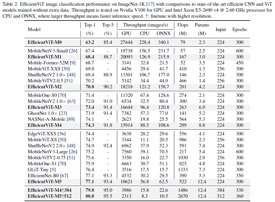 [2]より、ImageNet上での比較
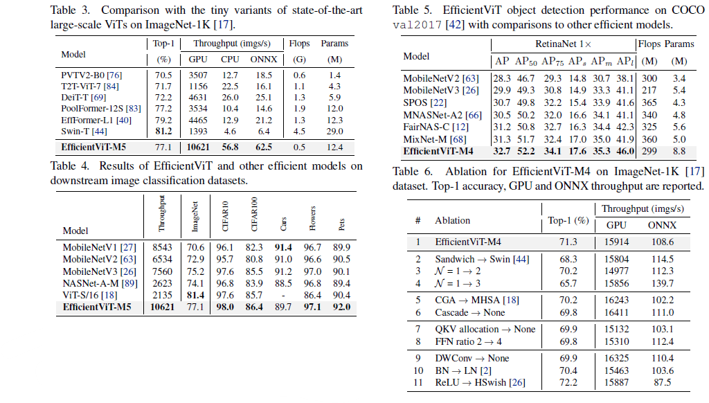 [2]より、他データセットでの比較とアブレーションスタディ
PoolFormerやEfficientFormerなどの競合と比べ速度効率が良いことが主張されている。ただImageNet top-1Acc 77.1はどのくらい実用的のかには疑問が残る。個人的にはHardSwishを使った場合に精度がかなり上がっているがONNXの推論速度が酷く落ちた所に面白さを感じた。また、通常のAttentionの方がGPU上では少し速いが、精度は落ちるというのも不思議。
実装
それぞれのモデルのブロックの実装を読んで、自作EfficientViTを作ってみる。
MITのモデル
以下のモデルのAttention部分を単純化してプレーンなtorchで書き直す。
まず使用するConv部分。timmではConvNormActに纏められているが、可視化時のわかりやすさのために活性化関数のありなしで分けた。
ConvNormAct/ConvNorm
from typing import Optional
import torch
import torch.nn as nn
import torch.nn.functional as F


class ConvNormAct(nn.Module):
    def __init__(
        self,
        in_channels: int,
        out_channels: int,
        kernel_size,
        stride=1,
        groups=1,
    ):
        super().__init__()
        self.conv = nn.Conv2d(
            in_channels,
            out_channels,
            kernel_size,
            stride=stride,
            groups=groups,
            padding=kernel_size//2,
            padding_mode="reflect",
        )
        self.norm = nn.BatchNorm2d(out_channels)
        self.act = nn.Hardswish()

    def forward(self, x):
        x = self.conv(x)
        x = self.norm(x)
        x = self.act(x)
        return x


class ConvNorm(nn.Module):
    def __init__(
        self,
        in_channels: int,
        out_channels: int,
        kernel_size,
        stride=1,
        groups=1,
    ):
        super().__init__()
        self.conv = nn.Conv2d(
            in_channels,
            out_channels,
            kernel_size,
            stride=stride,
            groups=groups,
            padding=kernel_size//2,
            padding_mode="reflect",
            bias=True
        )
        self.norm = nn.BatchNorm2d(out_channels)

    def forward(self, x):
        x = self.conv(x)
        x = self.norm(x)
        return x
class MBConv(nn.Module):
    def __init__(
        self,
        in_channels: int,
        out_channels: int,
        kernel_size=3,
        stride=1,
        mid_channels=None,
        expand_ratio=6,
    ):
        super().__init__()
        mid_channels = mid_channels or round(in_channels * expand_ratio)

        self.inverted_conv = ConvNormAct(in_channels, mid_channels, 1)
        self.depth_conv = ConvNormAct(mid_channels, mid_channels, kernel_size, stride=stride, groups=mid_channels)
        self.point_conv = ConvNorm(mid_channels, out_channels, 1)

    def forward(self, x):
        x = self.inverted_conv(x)
        x = self.depth_conv(x)
        x = self.point_conv(x)
        return x

class ResidualBlock(nn.Module):
    def __init__(
        self,
        main: Optional[nn.Module],
        shortcut: Optional[nn.Module] = None,
        pre_norm: Optional[nn.Module] = None,
    ):
        super().__init__()
        self.pre_norm = pre_norm if pre_norm is not None else nn.Identity()
        self.main = main
        self.shortcut = shortcut

    def forward(self, x):
        res = self.main(self.pre_norm(x))
        if self.shortcut is not None:
            res = res + self.shortcut(x)
        return res
ReLU Linear Attention部分(forward部分はtimmそのまま)
# Lightweight multi-scale linear attention
class LiteMLA(nn.Module):
    def __init__(
        self,
        in_channels: int,
        out_channels: int,
        heads: int or None = None,
        heads_ratio: float = 1.0,
        dim=8,
        scales=(5,),
    ):
        super().__init__()
        self.eps = 1e-5
        heads = heads or int(in_channels // dim * heads_ratio)
        total_dim = heads * dim

        self.dim = dim
        self.qkv = nn.Conv2d(in_channels, 3*total_dim, 1, padding_mode="reflect")
        self.aggreg = nn.ModuleList([
            nn.Sequential(
                nn.Conv2d(3*total_dim, 3*total_dim, scale, padding=scale//2, groups=3*total_dim),
                nn.Conv2d(3*total_dim, 3*total_dim, 1, groups=3*heads),
            )
            for scale in scales
        ])
        self.kernel_func = nn.ReLU()
        self.proj = ConvNorm(total_dim*(1+len(scales)), out_channels, 1)

    def _attn(self, q, k, v):
        dtype = v.dtype
        q, k, v = q.float(), k.float(), v.float()
        kv = k.transpose(-1, -2) @ v
        out = q @ kv
        out = out[..., :-1] / (out[..., -1:] + self.eps)
        return out.to(dtype)

    def forward(self, x):
        B, _, H, W = x.shape

        # generate multi-scale q, k, v
        qkv = self.qkv(x)
        multi_scale_qkv = [qkv]
        for op in self.aggreg:
            multi_scale_qkv.append(op(qkv))
        multi_scale_qkv = torch.cat(multi_scale_qkv, dim=1)
        multi_scale_qkv = multi_scale_qkv.reshape(B, -1, 3 * self.dim, H * W).transpose(-1, -2)
        q, k, v = multi_scale_qkv.chunk(3, dim=-1)

        # lightweight global attention
        q = self.kernel_func(q)
        k = self.kernel_func(k)
        v = F.pad(v, (0, 1), mode="constant", value=1.)

        out = self._attn(q, k, v)

        # final projection
        out = out.transpose(-1, -2).reshape(B, -1, H, W)
        out = self.proj(out)
        return out
Attention部分のみ表示してみる。
>>> LiteMLA(256, 256, 1)
LiteMLA(
  (qkv): Conv2d(256, 24, kernel_size=(1, 1), stride=(1, 1), padding_mode=reflect)
  (aggreg): ModuleList(
    (0): Sequential(
      (0): Conv2d(24, 24, kernel_size=(5, 5), stride=(1, 1), padding=(2, 2), groups=24)
      (1): Conv2d(24, 24, kernel_size=(1, 1), stride=(1, 1), groups=3)
    )
  )
  (kernel_func): ReLU()
  (proj): ConvNorm(
    (conv): Conv2d(16, 256, kernel_size=(1, 1), stride=(1, 1), padding_mode=reflect)
    (norm): BatchNorm2d(256, eps=1e-05, momentum=0.1, affine=True, track_running_stats=True)
  )
)
1つのEfficientViTBlockは、LiteMLA(context_module)とMBConv(local_module)の連結で構成されているので、上記のパーツをスケーリング通りに張り合わせることでMITのモデルが作れる。
MSResearchのモデル
Cascaded Group Attention、Local Window Attentionがかなり複雑。
ConvNorm/SEModule
from typing import Dict
import itertools

import torch
import torch.nn as nn


class SqueezeExcite(nn.Module):
    def __init__(self, channels):
        super().__init__()
        self.fc1 = nn.Conv2d(channels, channels//16, kernel_size=1)
        self.act = nn.ReLU(inplace=True)
        self.fc2 = nn.Conv2d(channels//16, channels, kernel_size=1)
        self.gate = nn.Sigmoid()
        return None

    def forward(self, x):
        x_se = x.mean((2, 3), keepdim=True)
        x_se = self.fc1(x_se)
        x_se = self.act(x_se)
        x_se = self.fc2(x_se)
        return x * self.gate(x_se)


class ConvNorm(nn.Sequential):
    def __init__(self, in_chs, out_chs, kernel_size=1, stride=1, pad=0, groups=1, bn_weight_init=1):
        super().__init__()
        self.conv = nn.Conv2d(in_chs, out_chs, kernel_size, stride, pad, groups, bias=False)
        self.bn = nn.BatchNorm2d(out_chs)
        torch.nn.init.constant_(self.bn.weight, bn_weight_init)
        torch.nn.init.constant_(self.bn.bias, 0)

    @torch.no_grad()
    def fuse(self):
        c = self.conv
        bn = self.bn
        w = bn.weight / (bn.running_var + bn.eps)**0.5
        w = c.weight * w[:, None, None, None]
        b = bn.bias - bn.running_mean * bn.weight / (bn.running_var + bn.eps)**0.5
        m = torch.nn.Conv2d(
            w.size(1)*self.conv.groups, w.size(0), kernel_size=w.shape[2:],
            stride=self.conv.stride, padding=self.conv.padding, groups=self.conv.groups)
        m.weight.data.copy_(w)
        m.bias.data.copy_(b)
        return m

class ConvMlp(nn.Module):
    def __init__(self, ch, mid_ch):
        super().__init__()
        self.pw1 = ConvNorm(ch, mid_ch, 1)
        self.act = torch.nn.ReLU()
        self.pw2 = ConvNorm(mid_ch, ch, 1, bn_weight_init=0)

    def forward(self, x):
        return self.pw2(self.act(self.pw1(x)))
おそらく、fuseによって学習後のBatchNormをConvの処理に加えて纏めている。学習時はそのままでなければ分散シフトを学習できない。
class CascadedGroupAttention(nn.Module):
    attention_bias_cache: Dict[str, torch.Tensor]
    def __init__(
            self,
            dim,
            key_dim,
            num_heads=8,
            attn_ratio=4,
            resolution=14,
            kernels=(5, 5, 5, 5),
    ):
        super().__init__()
        self.num_heads = num_heads
        self.scale = key_dim ** -0.5
        self.key_dim = key_dim
        self.val_dim = int(attn_ratio * key_dim)
        self.attn_ratio = attn_ratio

        qkvs = []
        dws = []
        for i in range(num_heads):
            qkvs.append(ConvNorm(dim//(num_heads), self.key_dim*2+self.val_dim, 1))
            dws.append(ConvNorm(self.key_dim, self.key_dim, kernels[i], groups=self.key_dim))
        self.qkvs = torch.nn.ModuleList(qkvs)
        self.dws = torch.nn.ModuleList(dws)
        self.proj = torch.nn.Sequential(
            torch.nn.ReLU(),
            ConvNorm(self.val_dim*num_heads, dim, 1, bn_weight_init=0)
        )

        points = list(itertools.product(range(resolution), range(resolution)))
        N = len(points)
        attention_offsets = {}
        idxs = []
        for p1 in points:
            for p2 in points:
                offset = (abs(p1[0] - p2[0]), abs(p1[1] - p2[1]))
                if offset not in attention_offsets:
                    attention_offsets[offset] = len(attention_offsets)
                idxs.append(attention_offsets[offset])
        self.attention_biases = torch.nn.Parameter(torch.zeros(num_heads, len(attention_offsets)))
        self.register_buffer('attention_bias_idxs', torch.LongTensor(idxs).view(N, N), persistent=False)
        self.attention_bias_cache = {}

    @torch.no_grad()
    def train(self, mode=True):
        super().train(mode)
        if mode and self.attention_bias_cache:
            self.attention_bias_cache = {}  # clear ab cache

    def get_attention_biases(self, device: torch.device) -> torch.Tensor:
        if torch.jit.is_tracing() or self.training:
            return self.attention_biases[:, self.attention_bias_idxs]
        else:
            device_key = str(device)
            if device_key not in self.attention_bias_cache:
                self.attention_bias_cache[device_key] = self.attention_biases[:, self.attention_bias_idxs]
            return self.attention_bias_cache[device_key]

    def forward(self, x):
        B, C, H, W = x.shape
        feats_in = x.chunk(len(self.qkvs), dim=1)
        feats_out = []
        feat = feats_in[0]
        attn_bias = self.get_attention_biases(x.device)
        for head_idx, (qkv, dws) in enumerate(zip(self.qkvs, self.dws)):
            if head_idx > 0:
                feat = feat + feats_in[head_idx]
            feat = qkv(feat)
            q, k, v = feat.view(B, -1, H, W).split([self.key_dim, self.key_dim, self.val_dim], dim=1)
            q = dws(q)
            q, k, v = q.flatten(2), k.flatten(2), v.flatten(2)
            q = q * self.scale
            attn = q.transpose(-2, -1) @ k
            attn = attn + attn_bias[head_idx]
            attn = attn.softmax(dim=-1)
            feat = v @ attn.transpose(-2, -1)
            feat = feat.view(B, self.val_dim, H, W)
            feats_out.append(feat)
        x = self.proj(torch.cat(feats_out, 1))
        return x


class LocalWindowAttention(torch.nn.Module):
    def __init__(
            self,
            dim,
            key_dim,
            num_heads=8,
            attn_ratio=4,
            resolution=14,
            window_resolution=7,
            kernels=(5, 5, 5, 5),
    ):
        super().__init__()
        self.dim = dim
        self.num_heads = num_heads
        self.resolution = resolution
        assert window_resolution > 0, 'window_size must be greater than 0'
        self.window_resolution = window_resolution
        window_resolution = min(window_resolution, resolution)
        self.attn = CascadedGroupAttention(
            dim, key_dim, num_heads,
            attn_ratio=attn_ratio,
            resolution=window_resolution,
            kernels=kernels,
        )

    def forward(self, x):
        H = W = self.resolution
        B, C, H_, W_ = x.shape
        # Only check this for classifcation models
        assert H == H_, f'input feature has wrong size, expect {(H, W)}, got {(H_, W_)}'
        assert W == W_, f'input feature has wrong size, expect {(H, W)}, got {(H_, W_)}'
        if H <= self.window_resolution and W <= self.window_resolution:
            x = self.attn(x)
        else:
            x = x.permute(0, 2, 3, 1)
            pad_b = (self.window_resolution - H % self.window_resolution) % self.window_resolution
            pad_r = (self.window_resolution - W % self.window_resolution) % self.window_resolution
            x = torch.nn.functional.pad(x, (0, 0, 0, pad_r, 0, pad_b))

            pH, pW = H + pad_b, W + pad_r
            nH = pH // self.window_resolution
            nW = pW // self.window_resolution
            # window partition, BHWC -> B(nHh)(nWw)C -> BnHnWhwC -> (BnHnW)hwC -> (BnHnW)Chw
            x = x.view(B, nH, self.window_resolution, nW, self.window_resolution, C).transpose(2, 3)
            x = x.reshape(B * nH * nW, self.window_resolution, self.window_resolution, C).permute(0, 3, 1, 2)
            x = self.attn(x)
            # window reverse, (BnHnW)Chw -> (BnHnW)hwC -> BnHnWhwC -> B(nHh)(nWw)C -> BHWC
            x = x.permute(0, 2, 3, 1).view(B, nH, nW, self.window_resolution, self.window_resolution, C)
            x = x.transpose(2, 3).reshape(B, pH, pW, C)
            x = x[:, :H, :W].contiguous()
            x = x.permute(0, 3, 1, 2)
        return x
このAttention部分(つまりサンドウィッチの具)のみを取り出して見てみる。
LocalWindowAttention(
    (attn): CascadedGroupAttention(
      (qkvs): ModuleList(
        (0-2): 3 x ConvNorm(
          (conv): Conv2d(64, 96, kernel_size=(1, 1), stride=(1, 1), bias=False)
          (bn): BatchNorm2d(96, eps=1e-05, momentum=0.1, affine=True, track_running_stats=True)
        )
      )
      (dws): ModuleList(
        (0): ConvNorm(
          (conv): Conv2d(16, 16, kernel_size=(7, 7), stride=(1, 1), padding=(3, 3), groups=16, bias=False)
          (bn): BatchNorm2d(16, eps=1e-05, momentum=0.1, affine=True, track_running_stats=True)
        )
        (1): ConvNorm(
          (conv): Conv2d(16, 16, kernel_size=(5, 5), stride=(1, 1), padding=(2, 2), groups=16, bias=False)
          (bn): BatchNorm2d(16, eps=1e-05, momentum=0.1, affine=True, track_running_stats=True)
        )
        (2): ConvNorm(
          (conv): Conv2d(16, 16, kernel_size=(3, 3), stride=(1, 1), padding=(1, 1), groups=16, bias=False)
          (bn): BatchNorm2d(16, eps=1e-05, momentum=0.1, affine=True, track_running_stats=True)
        )
      )
      (proj): Sequential(
        (0): ReLU()
        (1): ConvNorm(
          (conv): Conv2d(192, 192, kernel_size=(1, 1), stride=(1, 1), bias=False)
          (bn): BatchNorm2d(192, eps=1e-05, momentum=0.1, affine=True, track_running_stats=True)
        )
      )
    )
正直完全には理解できていない...
論文の要旨を思いっきり破壊してしまうが、このMemory-EffficientなAttentionで普通にViTのアーキテクチャを組んで計測してみたい。論文通りのスケーリングでは精度が大きく犠牲になっているが、単純に層が少ない分のロスに見えるので大規模化で通常のViTを超える精度効率も出せるかもしれない。
例えば次のように。
model = EfficientVitMsra(
    img_size=256,
    in_chans=3,
    num_classes=1000,
    embed_dim=(64, 128, 256, 512),
    key_dim=(16, 16, 16, 16),
    depth=(2, 2, 6, 2),
    num_heads=(4, 4, 4, 4),
    window_size=(7, 7, 7, 7),
    kernels=(7, 5, 3, 3),
    down_ops=(("", 1), ("subsample", 2), ("subsample", 2), ("subsample", 2)),
)
=================================================================================================
Layer (type (var_name))                         Input Shape               Output Shape
=================================================================================================
EfficientVitMsra (EfficientVitMsra)             [1, 3, 256, 256]          [1, 1000]
├─PatchEmbedding (patch_embed)                  [1, 3, 256, 256]          [1, 64, 16, 16]
│    └─ConvNorm (conv1)                         [1, 3, 256, 256]          [1, 8, 128, 128]
│    │    └─Conv2d (conv)                       [1, 3, 256, 256]          [1, 8, 128, 128]
│    │    └─BatchNorm2d (bn)                    [1, 8, 128, 128]          [1, 8, 128, 128]
│    └─ReLU (relu1)                             [1, 8, 128, 128]          [1, 8, 128, 128]
│    └─ConvNorm (conv2)                         [1, 8, 128, 128]          [1, 16, 64, 64]
│    │    └─Conv2d (conv)                       [1, 8, 128, 128]          [1, 16, 64, 64]
│    │    └─BatchNorm2d (bn)                    [1, 16, 64, 64]           [1, 16, 64, 64]
│    └─ReLU (relu2)                             [1, 16, 64, 64]           [1, 16, 64, 64]
│    └─ConvNorm (conv3)                         [1, 16, 64, 64]           [1, 32, 32, 32]
│    │    └─Conv2d (conv)                       [1, 16, 64, 64]           [1, 32, 32, 32]
│    │    └─BatchNorm2d (bn)                    [1, 32, 32, 32]           [1, 32, 32, 32]
│    └─ReLU (relu3)                             [1, 32, 32, 32]           [1, 32, 32, 32]
│    └─ConvNorm (conv4)                         [1, 32, 32, 32]           [1, 64, 16, 16]
│    │    └─Conv2d (conv)                       [1, 32, 32, 32]           [1, 64, 16, 16]
│    │    └─BatchNorm2d (bn)                    [1, 64, 16, 16]           [1, 64, 16, 16]
├─Sequential (stages)                           [1, 64, 16, 16]           [1, 512, 2, 2]
│    └─EfficientVitStage (0)                    [1, 64, 16, 16]           [1, 64, 16, 16]
│    │    └─Identity (downsample)               [1, 64, 16, 16]           [1, 64, 16, 16]
│    │    └─Sequential (blocks)                 [1, 64, 16, 16]           [1, 64, 16, 16]
│    │    │    └─EfficientVitBlock (0)          [1, 64, 16, 16]           [1, 64, 16, 16]
│    │    │    └─EfficientVitBlock (1)          [1, 64, 16, 16]           [1, 64, 16, 16]
│    └─EfficientVitStage (1)                    [1, 64, 16, 16]           [1, 128, 8, 8]
│    │    └─Sequential (downsample)             [1, 64, 16, 16]           [1, 128, 8, 8]
│    │    │    └─Sequential (res1)              [1, 64, 16, 16]           [1, 64, 16, 16]
│    │    │    └─PatchMerging (patchmerge)      [1, 64, 16, 16]           [1, 128, 8, 8]
│    │    │    └─Sequential (res2)              [1, 128, 8, 8]            [1, 128, 8, 8]
│    │    └─Sequential (blocks)                 [1, 128, 8, 8]            [1, 128, 8, 8]
│    │    │    └─EfficientVitBlock (0)          [1, 128, 8, 8]            [1, 128, 8, 8]
│    │    │    └─EfficientVitBlock (1)          [1, 128, 8, 8]            [1, 128, 8, 8]
│    └─EfficientVitStage (2)                    [1, 128, 8, 8]            [1, 256, 4, 4]
│    │    └─Sequential (downsample)             [1, 128, 8, 8]            [1, 256, 4, 4]
│    │    │    └─Sequential (res1)              [1, 128, 8, 8]            [1, 128, 8, 8]
│    │    │    └─PatchMerging (patchmerge)      [1, 128, 8, 8]            [1, 256, 4, 4]
│    │    │    └─Sequential (res2)              [1, 256, 4, 4]            [1, 256, 4, 4]
│    │    └─Sequential (blocks)                 [1, 256, 4, 4]            [1, 256, 4, 4]
│    │    │    └─EfficientVitBlock (0)          [1, 256, 4, 4]            [1, 256, 4, 4]
│    │    │    └─EfficientVitBlock (1)          [1, 256, 4, 4]            [1, 256, 4, 4]
│    │    │    └─EfficientVitBlock (2)          [1, 256, 4, 4]            [1, 256, 4, 4]
│    │    │    └─EfficientVitBlock (3)          [1, 256, 4, 4]            [1, 256, 4, 4]
│    │    │    └─EfficientVitBlock (4)          [1, 256, 4, 4]            [1, 256, 4, 4]
│    │    │    └─EfficientVitBlock (5)          [1, 256, 4, 4]            [1, 256, 4, 4]
│    └─EfficientVitStage (3)                    [1, 256, 4, 4]            [1, 512, 2, 2]
│    │    └─Sequential (downsample)             [1, 256, 4, 4]            [1, 512, 2, 2]
│    │    │    └─Sequential (res1)              [1, 256, 4, 4]            [1, 256, 4, 4]
│    │    │    └─PatchMerging (patchmerge)      [1, 256, 4, 4]            [1, 512, 2, 2]
│    │    │    └─Sequential (res2)              [1, 512, 2, 2]            [1, 512, 2, 2]
│    │    └─Sequential (blocks)                 [1, 512, 2, 2]            [1, 512, 2, 2]
│    │    │    └─EfficientVitBlock (0)          [1, 512, 2, 2]            [1, 512, 2, 2]
│    │    │    └─EfficientVitBlock (1)          [1, 512, 2, 2]            [1, 512, 2, 2]
├─SelectAdaptivePool2d (global_pool)            [1, 512, 2, 2]            [1, 512]
│    └─AdaptiveAvgPool2d (pool)                 [1, 512, 2, 2]            [1, 512, 1, 1]
│    └─Flatten (flatten)                        [1, 512, 1, 1]            [1, 512]
├─NormLinear (head)                             [1, 512]                  [1, 1000]
│    └─BatchNorm1d (bn)                         [1, 512]                  [1, 512]
│    └─Dropout (drop)                           [1, 512]                  [1, 512]
│    └─Linear (linear)                          [1, 512]                  [1, 1000]
===============================================================================================
Trainable params: 13,124,832
Non-trainable params: 0
Total mult-adds (M): 195.14
===============================================================================================
Input size (MB): 0.79
Forward/backward pass size (MB): 27.76
Params size (MB): 52.49
Estimated Total Size (MB): 81.04
===============================================================================================
感想
EfficientViTについて読んでみた。他にもEfficientFormerなどに見られるような「ViTを効率化する」ことはNNアーキテクチャ屋の大きな関心事だが、実用方面においては結局CNN化してしまっていると感じてしまう。今回の論文でも、ViTである必要性についてあまり議論されていないような気がした(というよりAttentionがConvの数よりとても少ない)。
MSResearchのモデルは非常に高速でMobileNetを使いたいシーンでは置き換えられる可能性が高いと思った。しかし通常のAttentionをもとに設計しているViT系モデルは入力解像度の変更ができないことも難点の一つで、MobileNetを使うシーン(リアルタイムの画面セグメンテーションなど?)を考えると実用的かどうかは疑問符がつく。
その意味で、MITのモデルは入力解像度も柔軟で、かなり現実的なラインの精度も出る良さがあると思った。しかし(これは完全に失礼な愚痴だが)構成部品とアーキテクチャがEfficientViTというより完全にEfficient CoAtNetで、ViTの論文だと思って読むとすこし肩透かしな気がする。と言いつつも、ReLU Linear Attentionの速度性能はかなり良いと感じたため、自分の性能評価遊びに使っていきたいと感じた。
Discussion