加算も乗算も使わない行列積の100倍高速な近似計算手法(Maddness)を自分で再実装して検証する!!!
Introduction
行列積という演算が機械学習/深層学習モデルの学習, 推論の計算に占める割合は非常に大きい。
昔僕が興味本位でやってみた実験なのだが、適当なTransformerの実装を持ってきてScaleDotProductAttentionというクラスの順伝播に含まれるmatmulというコードを消してみるだけで順伝播の計算量は90%削減できる。当然このモデルの出力は単語間の文脈が失われた意味のないものになるのだが、それだけに深層学習モデルに含まれる行列積の計算は重たい。
自宅のPCで深層学習を動かしていると真っ先にメモリ不足や性能不足といった問題に直面すると思う。ここで後者の性能不足という問題には、計算の大部分を占める行列積の近似計算をする(Approximate Multiplying Matrices, AMM) といったアプローチで取り組んでいる手法が存在する。
本記事では、Multiplying Matrices Without Multiplying (2021)という論文で提案されたMaddness(Multiply-ADDitioN-lESS)の手法について軽く触れたのち、一部を自力で再実装し、その速度を検証する。
Arxiv:
この手法の要点:
・Tall(縦に長い)かつDense(密)な、単一のメモリに乗り切る行列という仮定の上で成立 (i.e.: N >> D, M where N*D @ D*M.T)
・直積量子化(Product Quantization)をベースにした手法で、あらかじめ計算した行列積の結果をLUTに保存し再度それを参照することで、計算量がO(n)であるドット積の直接的な計算を回避し、1スレッドのCPUで通常通りの計算(OpenBLASと比較して?)と比較して、10~100倍の速度向上を達成した。
・一度エンコードをしたら以降使うのは比較命令と量子化された整数値の復元に使うaxpy!のみ (演算するデータ型がuint8であれば比較命令のみになる。)
・プロトタイプ -> Index値のエンコードにバイナリ回帰ツリーを用いる。これによってEncoding時間の性能を大幅に向上させた。
・求めた中心点をRidge回帰モデルによってさらに最適化する仕組みを導入。
・8bit量子化を適切な場所で使うことでCPUの並列処理性能を活用する
公式実装 (とても複雑なので覚悟して読んでください):
手法の概要
Maddnessは直積量子化という既存の近似手法に三つの改善点を導入した:
- MaddnessHashを用いた新しいLSH
- プロトタイプの最適化
- 8bit集約
だから基本的な戦略は直積量子化のそれと似通っている。まずは両者に共通する戦略から理解していくと捗る。
定式化
近似したい二つの密な行列をそれぞれ
行列積の計算が
-
プロトタイプの学習 (Prototype Learning) LSH(局所性鋭敏型ハッシュ)やKMeansなどの手法を用いて、行列AをC行ごとに切り出して、その特徴量に応じてK個のプロトタイプ(i.e.:
a\in\mathbb{R}^{N\times{C}} -
エンコード関数g(a)の作成 (Encoding Function) g(a)は与えられた行列a(プロトタイプと同じ形状)が、(1.)で求めたプロトタイプのうちどれに一番特徴が近いかを計算し、そのIndexを返す関数。
-
ハッシュ関数h(B)の計算 (Table Construction)
B A -
g(a)とh(B)の集約(Aggregation) 関数
f(g(a), h(B)) g(a) h(B)
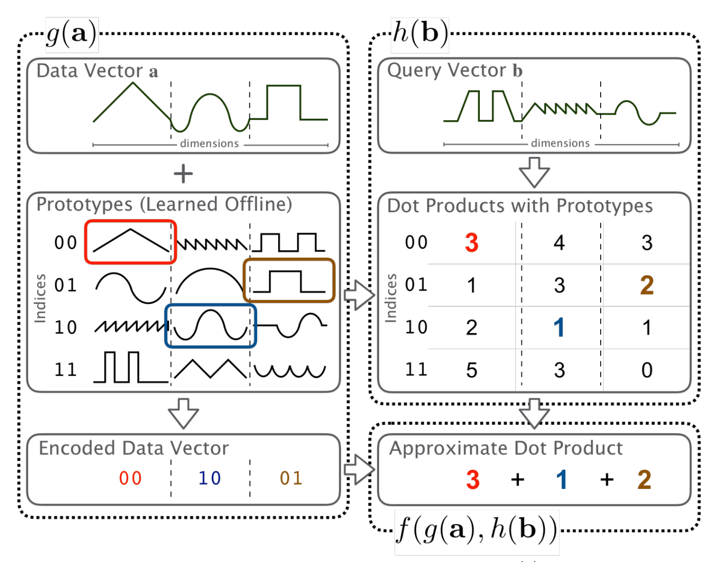
[Davis Blalock, John Guttag, Multiplying Matrices Without Multiplying (2021) [2]から引用]
図が複雑で時系列がよくわからないが、この手順は大きく二つに分かれている:
Encoder Part
- プロトタイプの学習
- エンコード関数の作成
- ハッシュ関数(LUT)の計算/構築
Decoder Part
- エンコード関数の計算
- g(a)とh(B)の集約
一度Encoder Partを計算すると、二回目以降の行列積計算を高速に行えるように最適化されたデータたちを得ることができる。それ以降はEncoder Partを呼び出すことはなく、新たな入力に対してDecoder Partのみを計算する流れになる。
プログラミングでいうとメモ化に近いイメージだと思う。メモ化は一度計算した値をHash関数に保存して再利用しようとするが、Maddnessや直積量子化などのLUTベースの手法は、以前行列積を計算した結果をなるべく小さい部分ごとに分けてLUTに保存し、二回目以降はその結果をもとに参照することを組み合わせて行列積を近似する。
そのためこの手法は一方の行列の値が固定でもう一方の行列が可変だが特徴量がある程度絞れるタスク、つまり機械学習/深層学習の推論と言ったタスクと非常に相性がいい。
推論に応用する
これを例えば機械学習モデルの推論に応用するならばこういう流れになる:
設定: 推論したいモデルはパラメーター行列
モデルのレイヤーごとに、予測する行列は
モデルの推論時という条件とこの近似手法はとても都合がいい。なぜならモデルの重みEncoding Partを実行するのが一番最適なのかは要検証といった感じみたい。)
繰り返すがとにかく一度
Bが固定なら、Maddnessを用いた時に占める計算量の大部分は
-
g(a) Bの各プロトタイプ -> Index値の計算) - LUTの参照
- 計算結果の集約時間
に収束する。
直積量子化 -> Maddness
Maddnessは直積量子化を元に以下の手法を新たに導入した。
・KMeansによるプロトタイプの分類→バイナリ回帰ツリーを元にしたLSH
・Ridge回帰を用いたプロトタイプの最適化 (New)
・8Bit Aggregation (8bit量子化をLSHとLUTそれぞれに適用) (New)
新しいエンコード関数g(x)
直積量子化ベースの手法はKMeansを用いてプロトタイプを分類しているが、KMeansは行列の特徴量を全て比較する(i.e.: Dが大きいほど露骨に計算量が増える)ため、高速な計算をするにはN, M >> Dとなる必要があるという厳しい仮定を設けることになっている。MaddnessはこのKMeansをバイナリ回帰ツリーを用いたLSHに置き換えることで条件をN >> D, Mに緩和し、さらに計算量を削減した。(Encoder Partで、行列Bは一切登場しない。)
バイナリ回帰ツリーは以下のような構造になっていて、各ノードをBucketと呼ぶ。(詳しくは実装編に記述します)
これを用いて、Aの各プロトタイプに対して特徴ごとに0~16のIndexを振り分ける。(ツリーの深さを表すnsplits=4の場合)
Encoder PartではそれぞれのBucketが持つパラメーターを最適化し、Decoder Partではそれを用いて、計算したい行列のプロトタイプを分類する。
Figure:                                |  t
              B(0, 1)                  | nth=0
         /----------------\            |
     B(1, 1)            B(1,2)         | nth=1
   /---------\        /---------\      |
B(2, 1)  B(2, 2)   B(2, 3)  B(2, 4)    | nth=2
       ...                ...          | ...
                                       | nth=nsplits
それぞれのBucketは以下の四つのスカラー値を持つ。
-
threshold
-
split-dim
-
scale
-
offset
-
2.と3. 4.はそれぞれプロトタイプの分類と、行列の量子化に用いられる。
nsplitsの値は基本的に4が計算量と精度のトレードオフから最適だとされている。
プロトタイプの最適化
作成したプロトタイプから、元の学習用行列を復元するときの誤差を小さくするように、プロトタイプを最適化する。
このタスクを解くためにはRidge回帰を用いていて、Encoding時間に占める割合はほぼ0になる。
8bit AggregationとLUTの量子化
上記のBucketの各地点の持つパラメーター
また、これからソースコードを読み解いていくとわかるが、LUTから行列積の結果を構築する部分について、若干の精度を犠牲にして加算命令の代わりに平均化命令を使うなど高速化のための工夫が散りばめられている。
まとめ
・二分木構造のLSHとメモ化のような計算をすることでドット積の再計算を減らした
。Ridge回帰を用いたプロトタイプ最適化
・LUTの検索には精度が不要なので、なるべくint8型に量子化することでcpuでもたくさんの並列化の恩恵を得られる。バケットの各地点が量子化のパラメーターを持つので表現力が高い。
再実装
ソースコードはこちら:
-
メインの部分
https://github.com/hikettei/cl-xMatrix/blob/main/source/amm/maddness.lisp -
Optimizing Prototypesの部分
https://github.com/hikettei/cl-xMatrix/blob/main/source/amm/least-squares.lisp
方針
・言語はCommon Lisp, 処理系はSBCLを用いる。ただしSIMD命令を使いたい部分は著者のC++実装から引用して、それをgccで共用ライブラリにコンパイルし、CFFIから呼び出すことにする。(公式の実装にはPythonとC++の二種類があるのだが、なぜか前者はDecoderの性能がよわよわで、後者はそもそもEncoderの実装がない。)
・Encoder関数の計算は行列の一部分だけを切り貼りできたりするライブラリがあると実装が楽なのだが、Common Lispでそれを可能にしてるのはほぼない(numericalsとpetalispあたりくらい?前者はSBCL依存で後者は癖がすごい強いのでこまる) そのためこれに合わせて行列演算ライブラリを自作した。
ほぼ自分用に作っているのでテストコードなどは不十分になっている。機会があったらAPIなどを整理してQuicklispに登録できるくらいの品質にしたい。
・Ridge回帰でプロトタイプを最適化する部分は、自作の深層学習ライブラリで実装する。cl-waffeもcl-xMatrixも行列のデータはCFFIのポインタとして保持されるため互換性がある。
両者APIや用語はなるべくNumpy/Torchと統一するよう心がけているが、利用経験のない方でもソースコードが読めるようになるべく適度コメントを振るようにした。
Encoder部分の実装
学習用行列→プロトタイプの分割
冒頭で述べた通り、学習用行列 learn-binary-tree-splits関数を適用する。以下の実装では各サブタイプをsubspaceという変数名で表現する。
(注釈: イメージしにくいと思うが、この分割方法は、TransformerのMultiHeadAttentionと同じ。単語のEmbeddingをnheads分割するイメージ)
  A_hat        P_1      P_2
 ===================================================
   D            C        C
  +++++       ++---    --++-
N +++++ =>  N ++---  N --++-
  +++++       ++---,   --++-,  ... (D/C)個数のsubspaceに分割
  ===================================================
  + ... ライブラリが見えている領域 (i.e.: numpyのviewで見える領域)
  - ... ライブラリからは見えない領域
ここで登場したC=16くらいがちょうどいい。
例として、C=4のような場合、学習用行列A_hatは以下のようにSliceされ、各領域でバイナリ学習木が回される。
binary-tree-splits(A_hat[:, 0~4])
binary-tree-splits(A_hat[:, 4~8])
binary-tree-splits(A_hat[:, 8~12])
...
binary-tree-splits(A_hat[:, (D-C)~D])
そのため、コードは以下の関数からスタートする。
init-and-learn-offline
(defun init-and-learn-offline (a-offline ;; Note: a-offline is destructed.
			       C
			       &key
				 (all-prototypes-out nil)
				 (nsplits 4) ;; the depth of binary-tree
				 (verbose t) ;; print log?
				 (K 16)      ;; the number of centroids (fixed)
			       &aux
				 (N (car (shape a-offline)))
				 (D (second (shape a-offline))))
  "
The function init-and-learn-offline clusters the prototypes, and then constructs the encoding function g(a).
Assertions:
  1. N must be divided by C (while the original impl doesn't impose it.)
  2. a-offline is a 2d-matrix.
Semantics:
=========================================================================
   D         C      C
  +++       +--    -+-
N +++ =>  N +--  N -+-  <- N*D Matrix is disjointed into N*C Matrix.
  +++       +--,   -+-  ... * (N/D), Binary-Tree-Split is applied into each visible area.
=========================================================================
Input:
  - a-offline The Training Matrix.
  - C fixnum  The Parameter Variable, C.
Return:
  - (values Prototypes List<Buckets> Loss)
"
  (declare (optimize (speed 3))
	   (type matrix a-offline)
	   (type fixnum N D C K))

  (assert (= (mod D C) 0) nil "Assertion Failed with (= (mod D C) 0). D=~a C=~a" N C)
  ;; with-view: Cut out the shape of matrix.
  ;; The visible-area is adjusted by modifying offsets.
  ;;    D        D
  ;;   +++    C +--
  ;; N +++ =>   +--
  ;;   +++      +--
  ;;
  ;; Symbols: + ... Visible, - ... Invisible

  ;; all-prototypes = (C, K, D)

  (let* ((step (/ D C))
	 (all-prototypes (or all-prototypes-out
			     (matrix `(,C ,K ,D) :dtype (dtype a-offline)))))

    (with-views ((a-offline* a-offline t `(0 ,step))
		 (all-prototypes* all-prototypes 0 0 `(0, STEP)))
      ;; a-offline*は以降形状が(N STEP)として扱われる。(ここにOffsetを加算するなどして高速に扱う領域を変える)
      (values
       (loop for i fixnum upfrom 0 below D by step
	     for c fixnum upfrom 0 below C
	     collect (let ((bucket (learn-binary-tree-splits a-offline* STEP :nsplits nsplits :verbose verbose)))
		       (with-cache (centroid `(1 ,STEP) :place-key :centroids)

			 ;; Update X-centroids
			 (with-bucket-clusters (id buck nsplits bucket)

			   (%fill centroid 0.0)
			   ;; 列ごとの平均値をcentroidとして使用する。
			   (col-means buck a-offline* centroid)

			   (with-views ((a* a-offline* `(:indices ,@(bucket-indices buck)))
					(c* centroid `(:broadcast ,(length (bucket-indices buck)))))
			     (%subs a* c*))

			   (incf-view! all-prototypes* 1 id)
			   (incf-offsets! all-prototypes* c)
			   ;; all-prototypes*は対角行列になる。Optimizing Prototypesで解決。

			   (%move (cl-xmatrix::reshape centroid `(1 1 ,STEP)) all-prototypes*)

			   (reset-offsets! all-prototypes*)
			   (incf-view! all-prototypes* 1 (- id))))
		       bucket)
	     unless (= i (- D step)) ;; 次のdo部分のためにOffsetを加算する
	       do (progn
		    (incf-view! all-prototypes* 2 step)
		    (incf-view! a-offline* 1 step)))
       all-prototypes))))
エンコード関数g(a)の学習
学習用行列を分割した各プロトタイプ
     C
   +++++
   +++++        C       C(dim=1)        /->  True, Bucketの右側に遷移
N  +++++ => 1 +++++ => 1 +☆+++ => (valの値より☆の値は大きいか?)
   +++++                                \->  False, Bucketの左側に遷移
   +++++

(あるBucketにてプロトタイプから行を一つ切り出し、valとdimの値で分類する図)
回帰ツリーの各ノードは、dim(整数値)とval(行列のデータ型と同じスカラー値)という二つの学習可能パラメーターを保持する。このようなデータ型をうまく表現するために、データ構造Bucketを導入する:
各Bucketはdimとvalのスカラー値を保持する。
Maddnessは下の図に示したような構造の決定木を学習して、プロトタイプ -> Indexを分類する回帰ツリーを獲得する。
Figure:                                |  t
              B(0, 1)                  | nth=0
         /----------------\            |
     B(1, 1)            B(1,2)         | nth=1
   /---------\        /---------\      |
B(2, 1)  B(2, 2)   B(2, 3)  B(2, 4)    | nth=2
       ...                ...          | ...
                                       | nth=nsplits
Common Lispでプログラミングするので、以下の構造体でBucketを表現した。
この時make-toplevel-bucketというコンストラクタで初期化する。そこから下に枝を増やしていく時は、コンストラクタmake-sub-bucketに分類されたindexの一覧indicesとツリーの深さを渡して新しく構造体を作る。ついでにBucketが利用するユーティリティーも定義する。
Bucket構造体とutils
(defstruct (Bucket
	    (:predicate bucket-)
	    (:constructor make-toplevel-bucket (indices &aux (tree-level 0) (id 0)))
	    (:constructor make-sub-bucket (indices tree-level id)))
  (tree-level tree-level :type fixnum) ;; ツリーの深さ
  (i id :type fixnum) ;; バケットのID(いらん)
  (scale  0.0 :type single-float) ;;
  (offset 0.0 :type single-float) ;; y=ax+bでsplit-valと行列を量子化してから計算する
  (threshold-quantized 0 :type fixnum) ;; 量子化されたsplit-val
  (index 0 :type fixnum)               ;; split-index
  (threshold  0.0 :type single-float)  ;; = split-val
  (threshold-candidates nil)           ;; 最適なsplit-indexを決めるための一時変数
  (next-nodes nil :type list) ;; 遷移先のノード, (cons A B)を取る
  (indices indices :type list)) ;; The list of indices of A which current bucket posses (C, D), D= 1 3 5 10 2 ... オリジナルの学習用行列から見て、Bucketが管轄する列のList

;; Bucketに含まれる各列の分散を求め、:axis=0で総和を求める。
(defmethod col-variances ((bucket Bucket) subspace &aux (N (length (bucket-indices bucket))))
  (declare (optimize (speed 3))
	   (type matrix subspace))
  (with-view (s* subspace `(:indices ,@(bucket-indices bucket)) t)
    (with-caches ((mu `(,(car (shape s*)) 1) :place-key :col-variances1)
		  (ex  (shape s*) :place-key :col-variances2)
		  (result `(1 ,(second (shape s*))) :place-key :sum-out1))
      (%fill result 0.0) ;; %sum is just broadcasting
      (%fill mu     0.0)

      (%sum s* :axis 1 :out mu)
      (%scalar-div mu (second (shape s*))) ;; mu <- mean(s*, axis=1)

      (with-view (mu mu t `(:broadcast ,(second (shape s*))))
	(%move s* ex) ;; ex <- s*
	(%subs ex mu) ;; ex <- ex - mu
	(%square ex)  ;; (xi - mu)^2
	(%scalar-div ex N) ;; ex <- ex / N
	(%sum ex :out result :axis 0)
	result))))

;; 各行の平均を求める関数
(defun col-means (bucket subspace out &aux (indices (bucket-indices bucket)))
  (declare (optimize (speed 3))
	   (type matrix subspace))
  (%scalar-div (%sum
		(view subspace `(:indices ,@indices))
		:out out
		:axis 0)
	       (max 1 (length indices))))
パラメーターの学習
Bucketの深さごとに(t=0, 1, 2, ...)各Bucketのdimとvalの値を求める。
ざっくりとした流れはこんな感じ:
任意の深さの各Bucketごとに、以下の操作を適用する。
- 任意のBucketに分類された行の一覧
(bucket-indices)から、後述の方法でLossを求める。この時、dim=0~Cで分類した時の全ての場合について損失を求め、軸ごとに一時変数に保存しておく。 - 全ての軸で損失を求めたら、その損失が最も少ない軸
best-trying-dimを求める。この値をdimとして使うことが最も優秀な分類機になると言うことになる。 -
dimと一致するvalをsubspaceから取り出し、それぞれ各地点のBucketのdimとvalにする。 -
dimとvalの値をもとに、回帰ツリーを一段階深くする。
各地点のBucketに対しての損失は以下のように求める:
その地点のBucketに分類された行の一覧(bucket-indices)の全ての行ごとに対して残差平方和(SSE)を用いて分類が上手くいってるかを評価する。損失が少なければ少ないほどそのBucketには同じような特徴の行が分類されてることになるはず。 (分類するベクトルが単語ベクトルとかなら、cos類似度にする方が妥当かもしれない。Encoding時間を気にしないならの話だが・・)
損失を求めるアルゴリズム

ごちゃごちゃと説明されるよりコードと動作を見ていただく方が理解しやすいと思います。
対応するコードはこちら:
-
learn-binary-tree-splitsプロトタイプごとにBucketのツリーを学習する関数 -
optimal-val-splits!目的のTree-Levelにたどり着くまで再帰+Lossの管理 -
optimal-splits-val現在の位置のBucketと与えられたdimでLossを求める -
cumulative-cols!各行でSSEを計算
learn-binary-tree-splits
(defun learn-binary-tree-splits (subspace STEP &key (nsplits 4) (verbose t) &aux (N (first (shape subspace))))
  "
The function learn-binary-tree-splits computes maddness-hash given subspace X.
=========================================
subspace:
   C      C
   ++     ++
 N ++   N ++ ... P_n ... Nth Prototype
   ++     ++
subspace will be splited into Bucket:
  C       C
  ++    N ++ <- B(tree-level, i)
N ++ ->
  ++    N ++ <- B(tree-level, i)
split-dim -> C
=========================================
4.1 Hash Function Family g(a)
 - MaddnessHash (BinaryTree)
 - 4.2 Learning the Hash-Function Parameters
 Let be B(t, i) the bucket which is helper structure where t is the tree's depth and is in the index in the node:
- Split Functions
- Loss: L(j, B) -> SSE
Figure:
              B(1, 1)                  | nth=0
         /----------------\            |
     B(2, 1)            B(2,2)         | nth=1
   /---------\        /---------\      |
B(3, 1)  B(3, 2)   B(3, 3)  B(3, 4)    | nth=2
                                       | ...
                                       | nth=nsplits
Inputs:
 - subspace Matrix[N, STEP]
 - C, D     Fixnum
 - nsplits The number of training, the original paper has it that setting 4 is always the best.
Thresholds - scalar, K-1
Split-Indices -
X = [C, (0, 1, 2, ... D)]
"
  (declare (optimize (speed 3))
	   (type matrix subspace)
	   (type fixnum STEP nsplits)
	   (type boolean verbose))

  (let ((buckets (make-toplevel-bucket
		  ;; B(1, 1) possess all the elements in the subspace.
		  (loop for i fixnum upfrom 0 below N
			collect i))))
    (with-cache (col-losses `(1 ,STEP) :dtype (matrix-dtype subspace) :place-key :losses1)
      (%fill col-losses 0.0)
      ;; Utils
      (macrolet ((maybe-print (object &rest control-objects)
		   `(when verbose (format t ,object ,@control-objects))))

	;; Training
	(dotimes (nth-split nsplits)
	  (maybe-print "== (~a/~a) Training Binary Tree Splits =========~%" (1+ nth-split) nsplits)

	  ;; heuristic = bucket_sse
	  (%fill col-losses 0.0)
	  (sumup-col-sum-sqs! col-losses buckets subspace)

	  (with-facet (col-losses* col-losses :direction :simple-array)
	    ;; Sort By [Largest-Loss-Axis, ... , Smallest-Loss-Axis]

	    (let* ((dim-orders (argsort col-losses* :test #'>))
		   (dim-size   (length dim-orders)))

	      (with-cache (total-losses `(1 ,dim-size) :place-key :total-loss)
		(%fill total-losses 0.0)
		;; Here, we tests all dims to obtain the best trying dim.
		;; depth = 0, 1, 2, ..., nth-split

		(loop for d fixnum upfrom 0
		      for dth in dim-orders
		      do (loop named training-per-bucket
			       for level fixnum from 0 to nth-split
			       do (when (optimal-val-splits! subspace buckets total-losses d dth level)

				    (return-from training-per-bucket))))

		;; total-losses = `(Loss1 Loss2 Loss3 ... LossN) where N=axis.
		;; (The next time nsplits training, The axis whose Loss is large is computes ahaed of time. <- considering col-losses)
		;;

		(let* ((best-trying-dim (first (argsort (convert-into-lisp-array total-losses) :test #'<)))
		       ;; Transcript dim -> sorted dim
		       (best-dim (nth best-trying-dim dim-orders)))
		  (declare (type fixnum nth-split))

		  ;; apply this split to get next round of buckets
		  (optimize-split-thresholds! buckets best-trying-dim best-dim nth-split subspace)

		  (optimize-bucket-splits!    buckets best-dim subspace))))))
	(when verbose
	  (maybe-print "Loss: ~a~%" (compute-bucket-loss buckets subspace)))
	buckets))))
optimal-val-splits!
(defun optimal-val-splits! (subspace bucket total-losses d dim tree-level)
  "The function optimal-val-splits! explores the bucket's nodes untill reaches tree-level, and update total-losses.
Input:
   d   - whichth axis of the total-losses to set the result.
   dim - the axis to be used.
Return:
   - early-stopping-p
"
  (declare (optimize (speed 3) (safety 0))
	   (type bucket bucket)
	   (type matrix subspace total-losses)
	   (type fixnum d dim tree-level))
  (if (= (bucket-tree-level bucket) tree-level)
      (multiple-value-bind (split-val loss) (compute-optimal-val-splits subspace bucket dim)
	(declare (type single-float split-val loss))

	(with-view (loss-d total-losses t 0)
	  (incf-offsets! loss-d 0 d)
	  (%scalar-add loss-d loss)
	  (let ((loss-d* (%sumup loss-d)))
	    (declare (type single-float loss-d*))

	    ;; Note: split-val[dim~0] <- dont forget to rev it.
	    ;; that is, dim is on the around way.

	    ;; candidates:
	    ;; dim-order[2] ... dim-order[1] dim-order[0]
	    ;; obtained by d
	    (push split-val (bucket-threshold-candidates bucket))
	    ;; Judge early-stoppig-p
	    (if (= d 0)
		nil
		(%all?
		 (%satisfies
		  (view total-losses t `(0 ,d))
		  #'(lambda (x) (< (the single-float x) loss-d*))))))))
      (let ((next-nodes (bucket-next-nodes bucket)))
	;; Explore nodes until reach tree-level

	(when (null next-nodes)
	  (error "optimal-val-splits! Couldn't find any buckets."))

	(let ((res1 (optimal-val-splits! subspace (car next-nodes) total-losses d dim tree-level))
	      (res2 (optimal-val-splits! subspace (cdr next-nodes) total-losses d dim tree-level))
	      (res3 (optimal-val-splits! subspace bucket total-losses d dim (bucket-tree-level bucket)))) ;; compute current-level node.
	  (or res1 res2 res3)))))
compute-optimal-val-splits
(declaim (ftype (function (matrix Bucket fixnum) (values single-float single-float)) compute-optimal-val-splits))
(defun compute-optimal-val-splits (subspace bucket dim
				   &aux
				     (D (second (shape subspace))))
  "The function optimal-val-splits tests all possible thresholds to find one minimizing B(tree-level, i).
Ref: Appendix C, Algorithm 3, Optimal Split Threshold Within a Bucket.
subspace - original subspace
"
  (declare (optimize (speed 3))
	   (type matrix subspace)
	   (type Bucket bucket)
	   (type fixnum dim))

  ;; when the bucket is empty.
  (when (or (null (bucket-indices bucket))
	    (< (length (bucket-indices bucket)) 2))
    (return-from compute-optimal-val-splits (values 0.0 0.0)))

  (let* ((indices (bucket-indices bucket))
	 (x       (view subspace `(:indices ,@indices) t)) ;; Cut out matrices which given bucket indicates.
	 (x-sort-indices      (sort-rows-based-on-col x dim))
	 (x-sort-indices-rev  (reverse x-sort-indices))
	 (N (length x-sort-indices)))
    (declare (type list x-sort-indices))

    (with-caches ((x-head `(,N ,D) :dtype (matrix-dtype subspace) :place-key :C1)
		  (x-tail `(,N ,D) :dtype (matrix-dtype subspace) :place-key :C2)
		  (s-out  `(,N 1)  :dtype (matrix-dtype subspace) :place-key :C3))
      (%fill s-out 0.0)

      ;; If the SSE error for all rows is small, then the Bucket has similar rows classified.
      ;; Note: Replace Loss Functions into: Cosine Simirality.
      ;; Which excepted to be working as if Reformer.
      ;; The assumption is that a single (dim, val) set isn't enough to cluster a embedding vector.
      (cumulative-sse! (view x `(:indices ,@x-sort-indices))     x-head)
      (cumulative-sse! (view x `(:indices ,@x-sort-indices-rev)) x-tail)

      ;; x-head = sses-head, x-tail = sses-tail
      ;; losses <- sses-head
      ;; losses[1:N-1] <- losses[1:N-1] + sses_tail[2:N]

      (%adds x-head x-tail)

      (%sum x-head :axis 1 :out s-out)

      ;; matrix->lisp-array conversations may contribute to low performance...
      ;; This could be reimplemented in C or define-vop.
      (with-facet (s-out* s-out :direction :simple-array)
	(let* ((best-idx (car (argsort s-out* :test #'<)))
	       (next-idx (min (the fixnum
				   (1- (the fixnum (car (shape subspace)))))
			      (the fixnum
				   (1+ best-idx))))
	       (col-idx1 (nth best-idx x-sort-indices))
	       (col-idx2 (nth next-idx x-sort-indices))
	       (c1 (view x col-idx1 dim))
	       (c2 (view x col-idx2 dim)))
	  (declare (type fixnum best-idx next-idx))
	  ;; c1 c2 = [1, 1]
	  ;; %sumup may slow... -> Add: mats-as-scalar
          ;; when dtype=uint?

	  ;; (values use-split-val use-loss)

	  (values (/ (+ (the single-float (%sumup c1))
			(the single-float (%sumup c2)))
		     2.0)
		  (the single-float (%sumup (view s-out best-idx)))))))))
cumulative-sse!
(defun cumulative-sse! (xp
			cumsses
			&aux
			  (N (car    (shape xp)))
			  (D (second (shape xp)))
			  (dtype     (dtype xp)))
  "Algorithm 4 Cumulative SSE. (Computes SSE Loss)
   Input: X [N D]
          out - the matrix to be overwritten with result. If nil, The function allocates a new matrix.
   Output: nil"
  (declare (optimize (speed 3))
	   (type index N D)
	   (type matrix xp cumsses))

  (with-caches ((cumX-cols  `(1 ,D) :dtype dtype :place-key  :cumsse-col1)
		(cumX2-cols `(1 ,D) :dtype dtype :place-key :cumsse-col2)
		(x          `(,N ,D) :dtype dtype :place-key :cognitious-x))
    (%fill cumX-cols 0.0)
    (%fill cumX2-cols 0.0)
    (%move xp x) ;; x-matrix's bug: move :indices-array into cognitious array.
    (with-views ((cxc cumX-cols 0 t)
		 (cxc2 cumX2-cols 0 t)
		 (x* x 0 t)
		 (cs cumsses 0 t))
      (%move x* cxc)
      (%move x* cxc2)
      (%square cxc2)

      (dotimes (i N)
	(let ((lr (/ (+ 2.0 i))))
	  (%adds cumX-cols x*)
	  (%adds cumX2-cols x*)
	  (let* ((meanX (%scalar-mul cumX-cols lr))
		 (mx    (%muls meanX cumX-cols))
		 (mx    (%scalar-mul mx -1.0)))
	    (%move cumX2-cols cs)
	    (%adds cs mx)))
	(incf-offsets! x* 1 0)
	(incf-offsets! cs 1 0))
      (reset-offsets! x*)
      (reset-offsets! cs))
    nil))
最適な閾値を求めたら、一番下のノードが持つvalとdimを更新して、各地点のBucketを一個下のtree-levelに分割していく。
optimize-bucket-thresholds!
(defun optimize-split-thresholds! (bucket d dth tree-level subspace)
  "Pick up index-th threshold-candiates, and use it as bucket's threshold."
  (declare (optimize (speed 3))
	   (type bucket bucket)
	   (type fixnum d dth tree-level))

  (when (= (bucket-tree-level bucket) tree-level)
    (setf (bucket-index bucket) dth)
    (setf (bucket-threshold bucket) (nth d (reverse (bucket-threshold-candidates bucket))))
    (learn-quantized-params! bucket subspace dth)) ;; 量子化のためのscaleとoffsetを計算する。(後述)

  (let ((buckets (bucket-next-nodes bucket)))
    (when buckets
      (optimize-split-thresholds! (car buckets) d dth tree-level subspace)
      (optimize-split-thresholds! (cdr buckets) d dth tree-level subspace)))
  nil)
Bucketの分割は以下のように行う。
その地点のbucket-indicesに含まれている各行に対して:
- 行の
dim番目の要素がvalより大きいか? -> 右側へ - 行の
dim番目の要素がvalより小さいか? -> 左側へ
optimize-bucket-splits!
(defun optimize-bucket-splits! (bucket
				best-dim
				subspace
				&aux
				  (right-idx (+ (* 2 (bucket-i bucket)) 1)) ;; 2x + 1
				  (left-idx (* (bucket-i bucket) 2))) ;; 2x
  "Todo: desc"
  (declare (optimize (speed 3))
	   (type bucket bucket)
	   (type matrix subspace)
	   (type fixnum best-dim right-idx left-idx))

  ;; if bucket-nodes = nil -> Create new
  ;; if t  -> Optimize the old one
  ;; Add: if indices = nil?

  (flet ((create-new-bucket (points id)
	   (make-sub-bucket points (1+ (bucket-tree-level bucket)) id))
	 (make-tflist-indices (tflist)
	   "(:tflist 1.0 0.0 1.0 ...) => (:indices 1 3 ...)"
	   (declare (type matrix tflist))

	   ;; Assertion: tflist isn't view-matrix
	   (assert (not (cl-xmatrix::matrix-projected-p tflist)) nil "make-tflist-indices: Assertion Failed because the given tflist is a view-object.")

	   ;; To Add: matrix but dtype=bit.
	   (loop for i fixnum upfrom 0 below (first (shape tflist))
		 if (= (the single-float (1d-mat-aref tflist i)) 1.0)
		   collect i)))

    (let* ((jurisdictions (bucket-indices bucket))
	   (x             (view subspace `(:indices ,@jurisdictions) best-dim))
	   (split-val     (bucket-threshold bucket))
	   (left-side-points)
	   (right-side-points))

      (with-caches ((mask     (shape x) :place-key :mask1)
		    (not-mask (shape x) :place-key :mask-not1))

	;; FIXME: conversation between lisp-array and matrix...

	;; Note: Having avoided using maddness-hash but using cons to express binary-tree-structure, I am wondering this semantics below is currect?

	;; x_ij >  val  -> assign to right
	;; x_ij <= val  -> assign to left

	;; left-side node can be obtained by:
	;; (car nodes)

	;; right-side node can be obtained by:
	;; (cdr nodes)

	(%>  x split-val :out mask)      ;; left
	(%<= x split-val :out not-mask)  ;; right

	(setq left-side-points  (make-tflist-indices mask))
	(setq right-side-points (make-tflist-indices not-mask))

	;; When left side child is supposed to be nil...?
	;; either is filled with copy of bucket
	(when (= (the single-float (%sumup mask)) 0.0)
	  (setq left-side-points (bucket-indices bucket)))

	;; When right side child is supposed to be nil...?
	(when (= (the single-float (%sumup not-mask)) 0.0)
	  (setq right-side-points (bucket-indices bucket)))

	(if (null (bucket-next-nodes bucket))
	    ;; If bucket is the end of node...
	    ;; => Creates a new bucket-tree.
	    (progn
	      (setf (bucket-next-nodes bucket)
		    (cons (create-new-bucket left-side-points left-idx)
			  (create-new-bucket right-side-points right-idx)))
	      nil)
	    ;; Otherwise -> Go deeper and update nodes.
	    (let ((nodes (bucket-next-nodes bucket)))
	      ;; Update Current Bucket -> Go Deeper

	      (setf (bucket-indices (car nodes)) right-side-points)
	      (setf (bucket-indices (cdr nodes)) left-side-points)

	      ;; Update Left-side
	      (optimize-bucket-splits!
	       (car nodes)
	       best-dim
	       subspace)

	      ;; Update Right-Side
	      (optimize-bucket-splits!
	       (cdr nodes)
	       best-dim
	       subspace)))))
    nil))
これを再起的に繰り返すことをnsplits回繰り返せばプロトタイプの数だけバイナリ回帰ツリーを得ることができる。
Bucketが保持するscaleとoffsetの学習
single-floatからuint8に量子化するためのパラメーターは各Bucketに含まれる列の最大と最小値から求めるため、学習用行列全体レンジに振り回されにくく、プロトタイプのレンジに依存する、そのため表現力が高くなっている。
Quantization and MaddnessHash

learn-quantized-param!
(defun learn-quantized-params! (bucket subspace best-dim)
  "Algorithm: Appendix B

  The function learn-quantized-param! computes the optimal parameters: scale and offset, and set it to the given bucket."
  (declare (optimize (speed 3))
	   (type matrix subspace)
	   (type fixnum best-dim))
  (multiple-value-bind (min-loss max-loss) (maxmin subspace best-dim)
    (let* ((sorts (sort (copy-list (bucket-threshold-candidates bucket)) #'<))
	   (min-val (car sorts))
	   (max-val (car (last sorts)))
	   (offset (/ (+ min-loss min-val) 2))
	   (upper-val (- (/ (+ max-loss max-val) 2) offset))
	   (l (log (/ 254.0 upper-val) 2))
	   (scale (expt 2 l))
	   (quantized-threshold (round (* (- (bucket-threshold bucket) offset) scale))))
      (setf (bucket-scale bucket) scale)
      (setf (bucket-offset bucket) offset)
      ;; y = af(x)+b
      (setf (bucket-threshold-quantized bucket) quantized-threshold)
      nil)))
(休憩)バイナリ回帰ツリーで遊んでみる
試しにベータ分布
ここでCommon Lispは実はそこらの言語より数値計算に強いことをステマするためにベータ分布を爆速でサンプリングするbeta-bb関数を用意した。
beta-bb関数
Generating Beta Variates with Nonintegral Shape Parametersの(> (min a b) 1.0)の場合の実装(BBアルゴリズム) Paper: https://dl.acm.org/doi/pdf/10.1145/359460.359482
(defun beta-bb (a0 a b)
  "
Generates beta variances for the case when (> (min a b) 1.0).
Algorithm: https://dl.acm.org/doi/pdf/10.1145/359460.359482"
  (declare (optimize (speed 3) (safety 0))
	   (type single-float a0)
	   (type (single-float 0e0) a b))

  (unless (>= (min a b) 1.0)
    (error "Assertion Failed with (min a b) > 1."))

  (let* ((alpha (+ a b))
  	 (beta  (sqrt (the (single-float 0e0)
			   (/ (- alpha 2.0)
			      (- (* 2.0 a b) alpha)))))
	 (gamma (+ a (/ beta)))
	 (r0 0.0)
	 (w0 0.0)
	 (t0 0.0))
    (labels ((next (&aux
		      (u1 (random 1.0))
		      (u2 (random 1.0))
		      (v (* beta (- (log u1) (log (+ 1.0 (- u1)))))))
	       (declare (type single-float u1 u2 v))

	       (setq w0 (* a (exp v)))
	       (setq r0 (- (* gamma v) 1.3862944))

	       (let* ((z (* u1 u1 u2))
		      (s (+ a r0 (- w0))))
		 (declare (type single-float z s))

		 (if (>= (+ s 2.609438) (* 5 z))
		     nil
		     (progn
		       (setq t0 (log z))
		       (if (>= s t0)
			   nil
			   t))))))
      (loop while (and
		   (next)
		   (< (+ r0
			 (* alpha (- (log alpha) (log (+ b w0)))))
		      t0)))

      (if (= a a0)
	  (/ w0 (+ b w0))
	  (/ b (+ b w0))))))
ちゃんとSBCLとかの数値計算に強い処理系を使っているなら高速に動く。
(time (dotimes (i 1000000) (beta-bb 5.0 5.0 2.0)))

Evaluation took:
  0.145 seconds of real time
  0.117017 seconds of total run time (0.116262 user, 0.000755 system)
  80.69% CPU
  334,088,524 processor cycles
  0 bytes consed
(defun test-binary-hashing-tree (&key (alpha 5.0) (beta 2.0))
  (let ((matrix (matrix `(128 16))))
    (%index matrix #'(lambda (i)
		       (beta-bb alpha alpha beta)))

    ;;(sb-ext:gc :full t)
    ;;(sb-profile:profile "CL-XMATRIX")
    (let ((bucket (learn-binary-tree-splits matrix 16)))
      (print-bucket-with-subspace bucket matrix))
    ;;(sb-profile:report)
    ;;(sb-profile:unprofile "CL-XMATRIX")
    (free-mat matrix)))
すると一番最後のプロトタイプの結果はこのようになり、そこそこ均等に分類できている。

この図の各Bucketが4つのスカラー値scale offset split-val thresholdを保持している。
プロトタイプの最適化
閑話休題、関数init-and-learn-offlineで得られる各プロタイプの中心点を集めた行列all-prototypesは、対角行列になっている。
これを深層学習ライブラリcl-waffeを用いて最適化する。
++++000000000
0++++00000000
00++++0000000
000++++000000
0000++++00000
00000++++0000
000000++++000
0000000++++00
00000000++++0
000000000++++

++++は各subspaceのcentroid (1 * K)
上のようなall-prototypeの列を組み合わせて、元の学習用行列
そのためにまず、学習して得た二分木を用いて学習用行列をIndex値から構成される行列にエンコードし、さらにそれをOnehot表現にエンコードする。これを行列Gとする。(深層学習ライブラリの損失関数がIndex値をそのまま与えることに対応してるなら、Onehotへのエンコードは必要ない。cl-waffe.nn:mseは対応してないので事前にエンコードしておく)
all-prototypesとし、
さらに加えて、このような最適化の手順を踏むことによって、オリジナルのsubspaceに存在しなかった領域のcentroidである、対角行列Pの両端の0の部分を最もらしい値で埋めることができる。
Encoder Partのうちプロトタイプ最適化が占める計算量は非常に小さく、事実上Overheadが0で計算できる。
OneHot表現へのエンコード, optimize-protos-with-ridge!
;; A-enc => one-hot表現に変換
(defun sparsify-and-int8-a-enc (a-enc K
				&aux
				  (N (car (shape a-enc)))
				  (C (second (shape a-enc)))
				  (D (* C K)))
    "
    returns X_binary from an encoded Matrix [N, C] vals (0-K)
    to (One-hot)
    [[0 0 0 ... 0 0 0]
     [0 0 1 ... 0 0 0]
     ...
     [0 0 0 ... 0 0 0]
     [0 0 0 ... 1 0 0]
     [0 0 0 ... 0 0 0]]
    "
  (declare (optimize (speed 3) (safety 0))
	   (type fixnum N C D K))
  ;; 疲れたのでカスすぎるコードを書くようになってしまった (ループの中でmatrixとsimple-arrayを扱うので並列処理性能がゴミ)
  (let ((out (make-array (* N D) :element-type '(unsigned-byte 256)))) ;; Each elements are at most K.
    ;; サイズが[K]のone-hotベクトルがC個(全てのプロトタイプごとに)ある
    (declare (type (simple-array (unsigned-byte 256) (*)) out))
    (dotimes (nth N)
      (dotimes (cth C)
        ;; %sumupは単純に総数が1の行列からスカラー値を得るために使っている。
	(let* ((code-left (round (the single-float (%sumup (view a-enc nth cth)))))
	       (dim-left  (+ (the fixnum (* K cth)) code-left)))
	  (declare (type fixnum code-left))
	  (setf (aref out (+ (the fixnum (* N nth)) dim-left)) 1))))
    out))

(defun optimize-protos-with-ridge! (protos x x-error buckets nsplits
				    &key
				      (lmd 1.0)
				      (required-loss 0.1)
				      (lr 1e-2)
				    &aux (K (expt 2 nsplits)))
   "minimize loss of |Y - Xw|^2 + alpha * |w|^2
    X is a orig-mat in my case.
    X [N, C * K]
    Y [N, C]
    W [D, C * K] -> W.T [C * K, D] later reshaped to [C, K, D] -> prototype's dimensons"
  (with-caches ((A-enc `(,(car (shape X)) ,K) :place-key :out-cache :dtype :uint8)

		(ofs    `(1 ,K) :place-key :offsets :dtype :uint8))
    (multiple-value-bind (scales offsets thresholds dims) (flatten-buckets buckets :nsplits nsplits)

      ;; エンコード関数(one-hotとは別の、maddness-encode関数)については次の項で触れる。
      (maddness-encode-c
       (matrix-vec X)
       (car    (shape X)) ;; N
       (second (shape X)) ;; D
       (matrix-vec dims)
       (matrix-vec thresholds)
       (matrix-vec scales)
       (matrix-vec offsets)
       K
       (matrix-vec A-enc))

      ;; Adding offsets = [0, 16, 32, ...] when K=16.
      (%index ofs #'(lambda (i) i)) ;; the equivalent to do arange(C) in numpy.
      (%scalar-mul ofs K)
      (%adds A-enc (view ofs `(:broadcast ,(car (shape X)))))

      (let ((x-binary (sparsify-and-int8-a-enc a-enc K)))
	;; x-binary = [N D]

	(let ((result
		(cl-xmatrix.amm.least-squares:optimize-with-ridge-regression
		 x-binary
		 x-error
		 (shape protos)
		 :alpha lmd
		 :required-loss required-loss
		 :lr lr)))
	  (declare (type cl-waffe:waffetensor result))
	  (let ((result (from-facet ;; cl-waffe's tensor -> x-matrix's matrix.
			 (cl-waffe:!shape result)
			 result
			 :direction
			 :foreign-waffe)))
	    (%adds protos result)
	    ;; todo: check how much improvement we got.
	    ;; プロトタイプ最適化によるLossの減り具合を可視化できるのだが、今回はめんどくさいので書いていない。 必要なら更新後のMSEを記述してください
	    ))))))
Common LispでのRidge回帰の実装(using cl-waffe)
;; In source/amm/least-squares.lisp

(in-package :cl-user)

(defpackage :cl-xmatrix.amm.least-squares
  (:use :cl :cl-waffe)
  (:export #:optimize-with-ridge-regression))

(in-package :cl-xmatrix.amm.least-squares)

(defmodel RidgeRegression (input-size output-size &key (alpha 0.1))
  :document "cl-waffeが扱う線形回帰モデル"
  :parameters ((linear (cl-waffe.nn:LinearLayer input-size output-size))
	       (alpha  (tensor alpha)))
  :forward ((x)
	    (call (self linear) x)))

(defmethod l2-regularization ((model RidgeRegression))
  "ペナルティー項を加算する"
  (let ((l2-reg (tensor 0.0)))
    (let ((linear (slot-value model 'linear)))
      (with-slots ((weight cl-waffe.nn::weight)) linear
	(!mul (ridgeregression-alpha model)
	      (!add l2-reg (!sqrt (!sum (!pow weight 2)))))))))

(deftrainer RidgeModel (input-size output-size alpha lr)
  :model          (RidgeRegression input-size output-size :alpha alpha)
  :optimizer      cl-waffe.optimizers:SGD
  :optimizer-args (:lr lr)
  :step-model ((x y)
	       (zero-grad)
	       (let* ((out  (call (model) x))
		      (loss (!add (!mean (cl-waffe.nn:mse out y))
				  (l2-regularization (model)))))
		 (backward loss)
		 (update)
		 loss))
  :predict ((x) (call (model) x)))

(defun optimize-with-ridge-regression (x-binary y proto-shape
				       &key
					 (alpha 1.0) ;; We fix λ=1.0
					 (lr 1e-2)
					 (required-loss 1.0) ;; Not anymore used.
				       &aux
					 (input  (car (cl-xmatrix:shape y)))
					 (output (second (cl-xmatrix:shape y)))
					 (D (/ (length x-binary) input)))
  "Minimizes The Function ||y - Xw||^2_2 + alpha * ||w||^2_2
Inputs:
  x-binary = [N, C*K] (simple-array)
  y        = [N C]    (matrix)
  alpha    = λ in original paprer. (single-float)

Return:
  The trained model's weight with reshaped into proto-shape.

Note: the code is so bad it is like a melting pot of sevaral type of matrices. ><"
  (declare (type simple-array x-binary)
	   (type single-float alpha lr)
	   (type cl-xmatrix:matrix y)
	   (ignore required-loss))

  (with-dtype :float
    ;; ここのデータ構造変換が頭悪い。(本当は各ライブラリでポインタを直接渡せるのだが時間がないので今回はこれで)
    (let ((model  (RidgeModel output D alpha lr))
	  (sparse (mgl-mat:array-to-mat x-binary))
	  (inputs (mgl-mat:array-to-mat
		   (cl-xmatrix:convert-into-lisp-array y))))

      ;; lrなどの設定が見当たらないので勘でやっている・・・
      (step-model
       model
       (!reshape (const inputs) `(,input t))  ;; Reshaped into: [N, output]
       (!reshape (const sparse) `(,input t))) ;; Reshaped into: [N, D]

      ;; weight [D, C * K]
      (let ((coeff (slot-value
		    (slot-value
		     (slot-value model 'model)
		     'linear)
		    'cl-waffe.nn::weight)))

	;; cl-waffeのlinear関数はTransposeを呼び出さないので, 論文の式とは違いTransposeしない(i.e. 既にcoeffはTransposeされている)
	(!reshape coeff proto-shape)))))
	```
プロトタイプ最適化は、序盤にトップレベルになると説明したinit-and-learn-offline関数の手順を踏んだ後に実行される。だからinit-and-learn-offline関数をラップして、さらにプロトタイプ最適化を実行する新たなトップレベル関数learn-prototypes-and-hash-functionを定義する。
learn-prototypes-and-hash-function
(defun learn-prototypes-and-hash-function (X C &key (nsplits 4) (verbose t) (optimize-protos t))
  (declare (optimize (speed 3))
	   (type matrix X)
	   (type fixnum C))

  (with-caches ((X-error (shape X) :dtype (dtype X) :place-key :x-err)
		(X-tmp   (shape X) :dtype (dtype X) :place-key :x-tmp))
    (%move X X-error)

    (multiple-value-bind (buckets protos)
	(init-and-learn-offline X-error C :nsplits nsplits :verbose verbose)

      ;; Displaying MSE Errors.
      (when verbose
	(let ((mse-orig
		(progn
		  (%move X X-tmp)
		  (%square X-tmp)
		  (meanup X-tmp)))
	      (mse-error
	 	(progn
		  (%move X-error X-tmp)
		  (%square X-tmp)
		  (meanup X-tmp))))
	  (declare (type single-float mse-orig mse-error))

	  (format t "== Report: ====~%MSE-Error / MSE-Orig -> ~a~%MSE-Error -> ~a~%MSE-Orig -> ~a~%"
		  (/ mse-orig mse-error)
		  mse-orig
		  mse-error)))

      ;; Optimizing Prototypes

      (when optimize-protos
        (optimize-protos-with-ridge! protos x x-error buckets nsplits))

      (values buckets protos))))
Maddness Hash
(注意:ここは自分の解釈が正しいかどうか自信がないです・・・)
CommonLispで学習した回帰ツリーはcons構造なので非常に入り組んでいる。SIMD演算による恩恵を受けるためこれを以下のアルゴリズムに従って、木構造を維持しながら一次元に直す。

==Buckets==========================================
              B(1, 1)                  | i=0
         /----------------\            |
     B(2, 1)            B(2,2)         | i=1
   /---------\        /---------\      |
B(3, 1)  B(3, 2)   B(3, 3)  B(3, 4)    | i=2
                                       | ...
                                       | i=nsplits
===================================================
↑これがプロトタイプ個ある。(Proto1 Proto2 Proto3...)

=> Maddness Hashに従うと
[Proto_1(Bucket_0), Proto_2(Bucket_0), ..., Proto_0(Bucket_1), ...]
にFlattenされる。

(Proto_n(Bucket_k) ... N番目のプロトタイプのk番目のBucket)
flatten-buckets
(defun gather-bucket (bucket slot tree-level)
  (declare (optimize (speed 3))
	   (type bucket bucket)
	   (type fixnum tree-level))
  (let ((result))
    (labels ((explore (bucket)
	       (with-slots ((children next-nodes) (tlevel tree-level))
		   bucket
		 (declare (type fixnum tlevel))
		 (when (= tree-level tlevel)
		   (push (slot-value bucket slot) result))
		 (when children
		   (explore (cdr children))
		   (explore (car children))))))
      (explore bucket)
      result)))

(defun flatten-buckets (buckets &key (nsplits 4))
  "[Proto_1(Bucket_0), Proto_2(Bucket_0), ...Proto_0(Bucket_1), ...]
Flatten buckets trained parameters following MaddnessHash."
  (labels ((collect (name)
	     (loop for i fixnum upfrom 0 below nsplits
		   nconc
		   (loop for b in buckets
			 nconc (gather-bucket b name i))))
	   (findsall (name dtype)
	     (let ((result (collect name)))
	       (from-facet
		`(1 ,(length result))
		result
		:direction :list
		:dtype dtype))))
    (values
     (findsall 'scale :float)
     (findsall 'offset :float)
     (findsall 'threshold-quantized :int)
     (findsall 'index :int))))
Lisp <-> C++の通信
以降定義する関数は計算のパフォーマンスに直結し、かつAVX2命令を使いたいので、CかC++を用いたい。C++なら論文の著者による公式実装が存在するので、そちらを使い、CFFIから呼び出すことにする。
cl-xMatrixは(matrix-vec matrix)のようにすることでCFFIが扱えるポインタを取り出せる。
CFFIで関数定義
(defcfun ("mithral_encode_fp32_t" maddness-encode-c) :void
  (X-pointer  (:pointer :float))
  (nrows       :int64)
  (ncols       :int)
  (splitdims   (:pointer :uint32))
  (all-splitvals (:pointer :uint8))
  (shifts      (:pointer :float))
  (offsets     (:pointer :float))
  (ncodebooks  :int) ;; nsplits
  (out-pointer (:pointer :uint8)))

(defcfun "mithral_scan_fp32_t" :void
  (encoded-mat (:pointer :uint8))
  (ncodebooks :int)
  (m :int)
  (luts (:pointer :uint8))
  (out  (:pointer :uint8)))

(defcfun "mithral_lut_fp32_t" :void
  (B (:pointer :float))
  (nrows :int)
  (ncols :int)
  (K     :int)
  (protos (:pointer :float))
  (out-offset-sum (:pointer :float))
  (out-scale      (:pointer :float))
  (tmp-lut-f32    (:pointer :float)) ;; tmp-lut-f32.shape == out.shape
  (out            (:pointer :uint8)))
高速エンコーダー mithral_encode_fp32_t
(休みが終わりそうなので急いで書いてます、今後追記するかも)
コードをそのまま僕の記事に貼り付けるのもどうかと思うので、該当するコードのURLだけ貼っておきます。
基本的にはCommon Lispで実装したBucketの分類のSIMD版。
特筆する部分としては、single-float型の行列Xはload_4xf32_as_32xepi8_or_epu8関数によって、学習で得た各Bucketのscaleとoffsetを用いて、uint8型に量子化されて計算される。
C/C++で愚直に書いた行列演算は#pragma SIMDをしたりimmintrin.hを用いてSIMD化しない限り、要素を一つ一つ計算するのでCPUはレジスタを持て余してしまい、CPUの性能をフルで使えないのだが、以下の関数を見ればわかるとおり行列のデータのサイズを落として一度の命令で多くの要素をレジスタに載せることで、一回の命令で24個の要素を並列処理できる。
template <bool Signed = true, bool SameOrder = true>
static inline __m256i load_4xf32_as_32xepi8_or_epu8(const float *x,
                                                    const __m256 &scales) {
  auto x0 = _mm256_mul_ps(_mm256_loadu_ps(x), scales);
  auto x1 = _mm256_mul_ps(_mm256_loadu_ps(x + 8), scales);
  auto x2 = _mm256_mul_ps(_mm256_loadu_ps(x + 16), scales);
  auto x3 = _mm256_mul_ps(_mm256_loadu_ps(x + 24), scales);
  return pack_ps_epi8_or_epu8<Signed, SameOrder>(x0, x1, x2, x3);
}
参考: 同等のCommon Lisp実装 (indexの計算がバグる + SIMD化されない)
(defun apply-hash-function! (A idx-out idx-tmp bucket)
  (declare (optimize (speed 3))
	   (type matrix A idx-out idx-tmp)
	   (type Bucket bucket))

  ;; Move: X-Axis
  ;; A[N, 1]は多分SIMD化されない・・・
  (with-slots ((v threshold) (children next-nodes)) bucket
    (declare (type single-float v))

    ;; apply for n times.

    ;; (car children) => left
    ;; (cdr children) => Right

    ;; A_ij >  v -> Assign to right: next_idx = 2i+1
    ;; A_ij <= v -> Assign to left : next_idx = 2i

    ;; MaddnessHash
    (with-unsafe ;; Shapeの形状を確認しない
      (%fill idx-tmp 0.0)
      (%>= A v :out idx-tmp) ;; FIXME: THE RESULT IS SINGLE_FLOAT...
      (%scalar-mul idx-out 2.0)
      (%adds idx-out idx-tmp))

    (when children
      ;; :tflistを使うとSIMD化されない
      (setq idx-tmp (%copy idx-tmp))

      (let ((left-indices  (tflist->indices idx-tmp))
	    (right-indices (tflist->indices idx-tmp :lognot t)))
	(declare (type list left-indices right-indices))
	;; Go left
	(unless (= (length left-indices) 0)
	  (apply-hash-function!
	   (view a       `(:indices ,@left-indices))
	   (view idx-out `(:indices ,@left-indices))
	   idx-tmp
	   (car children)))

	;; Go right
	(unless (= (length right-indices) 0)
	  (apply-hash-function!
	   (view a       `(:indices ,@right-indices))
	   (view idx-out `(:indices ,@right-indices))
	   idx-tmp
	   (cdr children))))
      nil)))

(defun maddness-encode (buckets
			prototypes
			A
			C
			&aux
			  (N    (first  (shape A)))
			  (D    (second (shape A)))
			  (STEP (/ D C)))
  "Buckets ... each subspace's bucket
prototypes ... prototypes obtained by training process.
A[N D] ... matrix to be encoded.

+++++
+++++
+++++"
  (declare (optimize (speed 3)) ;; safety 0
	   (type fixnum C N D STEP)
	   (type list buckets)
	   (type matrix A))

  ;; A[N, D] => A[N, C]
  ;; Prototype:[STEP, 0~4] -> 1,2,3,4,...16のIndexを振り分ける
  ;; FIXME: FLOAT _> INT
  (with-caches ((idxs    `(,N ,C) :place-key :encode-cache :dtype :float)
		(idx-tmp `(,N 1) :place-key  :idxs-tmp     :dtype :float))
    (%fill idxs 0.0)
    (%fill idx-tmp 0.0)
    ;; x's each proto -> idxs.
    (with-views ((idxs* idxs t 0)
		 (A*    A    t 0))
      ;; Move: Y axis
      (loop for i fixnum upfrom 0 below D by STEP
	    for c fixnum upfrom 0
	    do (let ((best-dim (bucket-index (nth c buckets))))
		 (incf-view! A* 1 best-dim)
		 (apply-hash-function! A* idxs* idx-tmp (nth c buckets))
		 (incf-view! A* 1 (- best-dim)))
	    unless (= i (- D step))
	      do (progn
		   (incf-view! A*    1 STEP)
		   (incf-view! idxs* 1 1))))
    idxs))
LUTの作成と量子化 mithral_lut_fp32_t
学習で得たprototypeとBの各行の行列積をあらかじめ計算し、それを量子化しLUTを作成する。
参考: 同等のCommonLispコード(未検証+SIMD化されない)
(defun maddness-quantize-luts! (lut)
  "Appendix A: Quantizing Look up Tables"
  ;;lut
  ;; tmp define for scalar
  (let ((max (max-multiple-axis=0and2 lut (second (shape lut))))
	(min (min-multiple-axis=0and2 lut (second (shape lut)))))
    (let* ((gaps (%subs max min))
	   (gap (argmax gaps))
	   (exponent (+ 1 (round (if (= gap 0.0)
				3.40e5
				(log gap 2)))))
	   (scale (expt 2 (- exponent)))
	   (scale (* scale (- 255.5 1e-10)))
	   (offsets (view (cl-xmatrix::reshape min `(1 ,(second (shape lut)) 1)) `(:broadcast ,(car (shape lut))) t `(:broadcast ,(third (shape lut))))))
      (with-caches ((lut-tmp       (shape lut) :dtype :float :place-key :ltmp)
		    (lut-quantized (shape lut) :dtype :uint8 :place-key :lut-q))
	(%move lut lut-tmp)
	(%subs lut-tmp offsets)
	(%scalar-mul lut-tmp scale)
	(%scalar-add lut-tmp 0.5)

	(%index lut-quantized
		#'(lambda (i) (print (1d-mat-aref lut i)) (round (print (1d-mat-aref lut-tmp i)))))
	(values lut-quantized scale (%sumup offsets))))))

(defun create-luts (protos B C K)
  (declare (type matrix protos b)
	   (type fixnum C K))
  ;; einsum(CKd, McD -> MCK)
  ;; M C K
  (with-cache (lut `(,(car (shape B)) ,C ,K) :place-key :lut-cache)
    (loop for i fixnum upfrom 0 below (car (shape B))
	  do (with-views ((lut* lut t t i)
			  (b* B i))

	       (maddness-lut! lut* b* protos)))
    (maddness-quantize-luts! lut)))
LUTの8bit集約 mithral_scan_fp32_t
エンコードされたIndex値の一覧とLUTから行列積の結果を構築する部分。
加算命令の代わりに平均化命令を用いることで、多少の精度と引き換えに速度を向上させている。
class MaddnessMatmul
Maddnessは扱うパラメーターが多すぎてごちゃごちゃになるのでMaddnessMatmulというクラスで全て管理することにする。(全て上記の関数を用いて計算するだけなので、読み飛ばしてもらって構わないです)
MaddnessMatmul
;; 次元数のチェックなどはないのでちょっと値間違えるとセグフォします

;; Usage:
;; (make-mithral N D M C nsplits)
;; -> #<MADDNESSMATMUL {1010867C63}>

;; N*D @ D*M
(defclass MaddnessMatmul ()
  ((N :initarg :N :type fixnum :reader mithral-n)
   (D :initarg :D :type fixnum :reader mithral-d)
   (M :initarg :M :type fixnum :reader mithral-m)
   (C :initarg :C :type fixnum :reader mithral-c)
   (nsplits :initarg :nsplits :type fixnum :reader mithral-nsplits)
   (K :type fixnum :reader mithral-k)
   (luts :type matrix   :writer write-luts)
   (protos :type matrix :writer write-protos)
   (buckets :type list :writer write-buckets)
   (A-enc :type matrix :writer write-a-enc)
   (B-mat :type matrix :writer write-b-mat)
   (alpha :type single-float :writer write-alpha)
   (beta  :type single-float :writer write-beta)
   (scales    :type matrix :writer write-scales :reader mithral-scales)
   (offsets   :type matrix :writer write-offsets :reader mithral-offsets)
   (splitdims :type matrix :writer write-splitdims :reader mithral-splitdims)
   (splitvals :type matrix :writer write-splitvals :reader mithral-splitvals)))

(defun make-mithral (N D M C nsplits)
  ;; To Add: Assertions
  (make-instance 'MaddnessMatmul
		 :N n
		 :D d
		 :M m
		 :C C
		 :nsplits nsplits))

(defmethod initialize-instance :after ((maddness MaddnessMatmul) &key &allow-other-keys)
  (with-slots ((K K) (nsplits nsplits)) maddness
    (setf K (expt 2 nsplits))))
set-a-offline
学習用行列を引数に取り、プロトタイプに分割、回帰ツリーの学習、プロトタイプ最適化・・・を行う。
set-a-offline
(defmethod set-a-offline ((maddness MaddnessMatmul) a-offline)
  ;; 二分木を学習
  (multiple-value-bind (buckets protos) (learn-prototypes-and-hash-function a-offline (mithral-c maddness))
    ;; 学習した結果を、一次元の配列に直す
    (multiple-value-bind (scales offsets thresholds split-dim)
	(flatten-buckets buckets)

      (write-protos  protos maddness)
      (write-buckets buckets maddness)

      (write-scales    scales maddness)
      (write-offsets   offsets maddness)
      (write-splitdims split-dim maddness)
      (write-splitvals thresholds maddness))))
set-a
set-a-offlineで求めたエンコード関数を用いて、A(計算のたびに毎回変更する方の行列)をエンコードし、最も近いプロトタイプのIndexの一覧を占めるuint8型の行列を作成し、slotA-encに保持する。
set-a
(defmethod set-a ((maddness MaddnessMatmul) A)
  ;; Encode A
  (declare (optimize (speed 3))
	   (type matrix A))
  (with-caches ((out `(,(car (shape A)) ,(mithral-k maddness)) :place-key :out-cache :dtype :uint8)
		(offsets `(1 ,(mithral-k maddness)) :place-key :offsets :dtype :uint8))

    (maddness-encode-c
     (matrix-vec a)
     (car    (shape A)) ;; N
     (second (shape A)) ;; C
     (matrix-vec (mithral-splitdims maddness))
     (matrix-vec (mithral-splitvals maddness))
     (matrix-vec (mithral-scales maddness))
     (matrix-vec (mithral-offsets maddness))
     (mithral-k maddness)
     (matrix-vec out))

    ;; 列ごとのオフセットを加算
    (%index offsets #'(lambda (i) i))
    (%scalar-mul offsets (mithral-k maddness))

    ;; offsets = [ 0  16  32  48  64  80  96 112 128 144 160 176 192 208 224 240]
    (%adds out (view offsets `(:broadcast ,(car (shape A)))))
    (write-a-enc out maddness)
    nil))
set-b
メソッドset-bは、set-a-offlineの結果と行列BからLUTを作成、量子化する。
set-b
(defmethod set-b ((maddness MaddnessMatmul) B)
  ;; Create_Luts from B
  (multiple-value-bind (luts alpha beta)
      (maddness-create-and-quantize-luts
       (slot-value maddness 'protos)
       B
       (mithral-c maddness)
       (mithral-k maddness))
    (write-luts luts maddness)
    (write-alpha alpha maddness)
    (write-beta beta maddness)
    (write-b-mat B maddness)
    nil))
calc-matmul
set-a-offline, set-a, set-bの情報を用いて行列積を近似する。
calc-matmul
;; LUTを読み取った結果から、alphaとbetaを用いて、元のfp32行列に復元する。
(declaim (ftype (function (matrix single-float single-float fixnum) matrix) restore-fp32-matrix))
(defun restore-fp32-matrix (matrix alpha beta C &aux (upcast-every 32))
  "Computes y=ax+b"
  (declare (optimize (speed 3) (safety 0))
	   (type single-float alpha beta)
	   (type fixnum C))

  ;; upcast_every = 32 is fixed.
  (with-cache (m* (shape matrix) :dtype :float :place-key :m1)
    ;; Rewrite it in C cuz it slow
    (%index m* #'(lambda (i &aux (read-lut (1d-mat-aref matrix i)))
		   (declare (type fixnum read-lut))
		   ;; 自作ライブラリはuint8 -> single-floatのキャストができないので、Common Lisp実装にしているが、SIMD化が効かないので非常に遅い。ベンチマーク時はここを除外する。
		   ;; 僕も色々試行錯誤してこれが一番答えに近かったが、なぜこれで復元できるのかはよくわからん・・・
		   (let ((bias (the single-float (* (/ C 4.0)
						    (log upcast-every 2)))))
		     (* -1.0 (+ (/ (+ read-lut bias) alpha) beta)))))
    m*))


(defparameter *benchmark-mode* nil "If t, the ugly part restore-fp32-matrix is ignored.")

(defmethod calc-matmul ((maddness MaddnessMatmul)
			&aux
			  (M (mithral-m maddness))
			  (N (mithral-n maddness)))
  ;; Scan
  (with-cache (out `(,N ,M) :place-key :matmul-result :dtype :uint8)
    (mithral-scan-fp32-t
     (matrix-vec (slot-value maddness 'a-enc))
     (mithral-k maddness)
     M
     (matrix-vec (slot-value maddness 'luts))
     (matrix-vec out))
    (unless *benchmark-mode*
      (restore-fp32-matrix
       out
       (slot-value maddness 'alpha)
       (slot-value maddness 'beta)
       (slot-value maddness 'C)))))
試してみる
MaddnessMatmulのメソッドのうち、Encoder/Decoderの対応はこんな感じ
Encoder Part (今回はこっちのベンチマークはしない。):
set-a-offline
set-b
Decoder Part (ここをベンチマークで使う):
set-a
calc-matmul
一度Encoder Partを計算したら以降のDecoder Partは爆速で動く。
Encoder Partはほぼ自作の行列演算ライブラリで実装したが(何せライブラリは作り始めてからまだ一ヶ月だしテストコードが少ないので)Numba実装などに比べるとパフォーマンスも安定性も非常に劣る。 MaddnessのEncoding関数も非常に高速なのでできればそちらも含めてせっかくならそちらもベンチマークを取りたかったのだが、またいつかの機会にする。(ちなみにsb-profile:profileの結果からは、CFFIを介したメモリの割り当てが全体の80%くらい計算時間を占めている...)
;; Tested on REPL.

(defparameter N 256)
(defparameter D 64)
(defparameter M 32)
(defparameter C 16)
(defparameter nsplits 4) ;; nsplits=4 is fixed.

(defparameter maddness (make-mithral N D M C nsplits))

(defparameter a-offline (matrix `(,N ,D)))
(defparameter a (matrix `(,N ,D)))
(defparameter b (matrix `(,M ,D)))

(%index a-offline #'(lambda (i) (random 1.0)))
(%index a #'(lambda (i) (random 1.0)))
(%index b #'(lambda (i) (random 1.0)))

(set-a-offline maddness a-offline)
(set-b maddness b)

(calc-matmul maddness)

;;<Matrix :float :shape (256 32) :view (T T) :visible-shape (256 32)
;; :vec ((16.217566  16.28031   ~ 15.715605  15.590115)
;;                   ...
;;       (16.092075  15.590115  ~ 16.15482   15.90384))>
速度比較のために、同じ計算を同じ値のままOpenBLASで実行する関数を定義する。
(defun matmul-openblas (a b)
  (cl-waffe:with-no-grad
    (with-facets ((a* a :direction :simple-array)
		  (b* b :direction :simple-array))
	(let ((a* (cl-waffe:!reshape (cl-waffe:const a*) (shape a)))
	      (b* (cl-waffe:!reshape (cl-waffe:const b*) (shape b))))
	  (time (cl-waffe:!matmul a* (cl-waffe:!transpose b*)))))))

(matmul-openblas a b)
#Const(((16.39... 16.51... ~ 15.55... 13.66...)
                 ...
        (16.33... 14.94... ~ 15.22... 13.87...)) :dtype :float :shape (256 32) :backward NIL)
復元された値はいい線を言っているのだが、どうも公式のNumba実装のものと比べて、uint8->single-floatの復元がうまくいっていないように感じる・・・(公式実装はもっと精度が高いはず)
深層学習や機械学習などのタスクにおいて、モデルが扱う行列は大抵確率分布だと思う。その場合、モデル全体にMaddnessを適用しているなら、行列全体の値の大小さえ入れ替わらないならOpenBLASの計算と多少値が異なっても事実上問題はない。それを満たしているという意味では実験は成功だと思う。(ちなみに:今回は触れないが元論文では近似精度の保証が不等式で与えられている)
計算速度についても見ていこう。以下はN=256の場合である。
;; OpenBLASでベンチマーク用の関数
;; 注意: cl-waffeのmatmulは、!transposeによるオーバーヘッドは0になる。
(defun matmul-benchmark-openblas (a b)
  (cl-waffe:with-no-grad
    (with-facets ((a* a :direction :simple-array)
		  (b* b :direction :simple-array))
	(let ((a* (cl-waffe:!reshape (cl-waffe:const a*) (shape a)))
	      (b* (cl-waffe:!reshape (cl-waffe:const b*) (shape b))))
	  (time (dotimes (i 1000) (cl-waffe:!matmul a* (cl-waffe:!transpose b*))))))))


(let ((*benchmark-mode* t))
      (time (dotimes (i 1000) (calc-matmul maddness))))
Evaluation took:
  0.006 seconds of real time
  0.006185 seconds of total run time (0.006046 user, 0.000139 system)
  100.00% CPU
  14,539,798 processor cycles
  32,512 bytes consed

(matmul-benchmark-openblas a b)
Evaluation took:
  0.685 seconds of real time
  0.345943 seconds of total run time (0.105684 user, 0.240259 system)
  [ Run times consist of 0.169 seconds GC time, and 0.177 seconds non-GC time. ]
  50.51% CPU
  1,579,923,574 processor cycles
  37,357,408 bytes consed
この場合はN=256で、仮定を十分に満たしているのかはわからないが、噂通りOpenBLASの約113.83倍高速に計算できている。注意してほしいが、Maddnessが有効になる局面というのは非常に限定的なので、一概にどっちが優れているみたいな話ではない。
ちなみに、cl-waffe(OpenBLAS)のmatmul関数のベンチマークは下にある。どのスケールにおいてもNumpy(MKL)とほぼ変わらない。
Experiments
計算速度
set-aとcalc-matmulの合計時間とOpenBLAS(OPENBLAS_NUM_THREADS=1)で検証する。
ソースコード:
環境
$ export OPENBLAS_NUM_THREADS=1
計算環境:

注意点:
- uint8->single-floatへの復元は自作ライブラリだとSIMD化ができないので、今回は除外する。Maddnessの結果は実際にはもう少し遅くなるかもしれない。(いうても定数時間が足されるだけだと思う)
- 実行時間のうち関係ない部分のgc時間を除外するため、実行前に
(sb-ext:gc :full t)をしておく。
Result1
変数は以下の通り
N=64, 128, 256, 512, 1024, 2048
D=64, M=32, C=16
try_n=1000
結果1 (Logscaled)

MaddnessとOpenBLASがどのスケールで有効なのかを調べるためにx, y軸で対数を取ったグラフを用意した。
N<128の範囲では、Maddnessの仮定N >> D, Mに反しているのでOpenBLASのよりも遅い。それ以降についてはOpenBLASよりも傾きが緩やかになっていて、高速に計算できていることがわかる。
結果1 (通常)

MaddnessがOpenBLASの何倍ほど早いかを調べるために、対数を取っていないバージョンのグラフも用意した。試行回数が1000回なので、スケールが小さい範囲では関数呼び出しのオーバーヘッドなどが行列積の計算時間より大きくなり、そのせいで多少値がおかしいかもしれないが、スケールが大きくなるにつれてMaddnessが有利になっていることがわかる。
計算精度
ここまで読んでいただいて本当に申し訳ないのですが、時間がないので推論での検証はまたいつかに持ち越そうと思います・・・
ですが計算精度や推論への応用に関して、参考になる文献を紹介させてください。
こちらのリポジトリにリファクタリングされた実装、様々なモデルに適用した時のベンチマーク、精度検証や、CUDAでの実装、手法の概要などが綺麗にまとめられているので、もしもっと深掘りしたいと思う方がいましたらこちらが参考になると思います。まずは手元でMaddnessを試してみたいという場合にも、すごく役立つと思います!
モデルの精度に関する資料を読んでいただければわかると思いますが、脳死でMaddnessに置き換えると必ずしもうまくというわけではなく、Cのパラメーターの設定やどこでLUTを構築するか・・・など、用途に応じて考えることが多く、その精度も効果が限定的なので、いまだにMaddnessは推論の高速化における主流とはなっていません。
まとめ
本記事も元論文も「加算命令もない100倍高速な行列積演算」を謳うという大変挑発的なタイトルになっていて、この手法が好ましくない意図で広まることを避けたいので断言しておきますがMaddnessは既存のOpenBLAS/MKLを置き換えるものでもありませんし、StrassenのアルゴリズムやCoppersmith–Winogradのアルゴリズムのように、とりあえずライブラリに導入して高速に動くといったこともありません。
MaddnessはOpenBLASの100倍高速に動く局面は限定的ですし、その精度についても十分ではないかもしれません。CUDAへの応用や更なる精度の向上など、課題はたくさん残っていますので、あくまで今後の研究に期待したいな〜くらいで受け止めていただくのが健全だと個人的に思います。
GWも終盤戦になり、執筆時点でもう最終日なので急いで記事を書き上げました。後半へ進むにつれて文章が雑になってしまい申し訳ないです。
拙い文章でしたが記事を最後まで読んでいただきありがとうございます!最後のReferencesに参考になる文献をまとめておきましたので、これ以上深掘りしたいという方がいましたらぜひご活用ください!
実装上の課題
・自前実装のEncoding関数が不安定ですぐFLOATING-POINT-OVERFLOWする。本家の実装はそんなことないので原因を見つけて修正したい...
・自前実装のEncoder部分がめちゃくちゃ遅い。本来MaddnessのEncoding関数は爆速なので、時間がある時にコードを最適化したい。ちなみにNumbaで適当に実装し直すだけで100倍くらい速くなります。
・大人しくJuliaで書き直す。
反省点
・逆張りしてCommon Lispでフルスクラッチで作らないでも、初めから素直にPythonとかJuliaを使えばよかった。したら実装に一週間もかからなかったし、GWもたくさん遊べた。
追記(2023/05/11)
結局Numba/Python/C++使って書き直してます (Readme.mdなどの整備はもう少し待ってください!!!)↓
(毎度の如く)時間がなくて記事が殴り書きになってしまったので、時間を見つけてもう少しゆっくり検証したいです。特にResNetや言語モデルを動かしたときの精度低下が気になります。。。
References
[1] https://github.com/joennlae/halutmatmul オリジナルのコードのリファクタリングや、CUDA Kernel版, 学習/推論で実験した結果などが載っている。わかりやすいPDFもたくさんあるのですごく役に立った。
[2] https://arxiv.org/pdf/2106.10860.pdf
[3] https://arxiv.org/pdf/1703.05160.pdf
[4] https://speakerdeck.com/ryoherisson/multiplying-matrices-without-multiplying 日本語のスライド, 僕の文字ばっかりな説明だとイメージがつきにくいと思うが、こちらは図を用いて説明しているので参考になると思う。
Discussion