🔰
【MCMC法①】PythonでMCMCを実装してみよう

2025/04/25に公開
通常のモンテカルロ法だと分布の次元が増えるにつれてサンプルがほとんど棄却されてしまうという「次元の呪い」がある。
このような問題を改善できるのが「MCMC（マルコフ連鎖モンテカルロ法）」である。

前回の試行結果を用いて、次の試行を確率的に改善していくというのが大きなMCMCの流れである。

 MCMCの流れ Metropolis-Hastings法初期値 \theta を適当に決める
乱数で今の \theta から新しい \theta_{new} を探す。（マルコフ連鎖）
次の条件式を判定する。

p(\theta_{new}|D)>p(\theta|D)
真の場合は状態を更新。偽の場合はある程度の確率で受容。

受容確率\approx1\rightarrowほぼ必ず移動受容確率<1\rightarrow少しだけの確率で移動
2~4を繰り返す。

 Pythonで実装してみるGitHubのリンク：https://github.com/Go-Morishita/mcmc-python
初期値 \theta を適当に決めるx = 0.5 # 初期値
乱数で今の \theta から新しい \theta_{new} を探す。（マルコフ連鎖）

提案分布は正規分布とする。x_proposal = np.random.normal(x, proposal_std)
次の条件式を判定する。
p(\theta_{new}|D)>p(\theta|D)acceptance_ratio = target_dist(x_proposal) / target_dist(x)
真の場合は状態を更新。偽の場合はある程度の確率で受容。if np.random.rand() < acceptance_ratio:
    x = x_proposal

 全体のコードimport numpy as np
import matplotlib.pyplot as plt

def target_dist(x):
    return np.sin(2 * np.pi * x) + 1

samples = []
num_steps = 1000000
x = 0.5 # 初期値
proposal_std = 0.1 # ジャンプ幅

for i in range(num_steps):
    # 今回は正規分布を提案分布とする
    x_proposal = np.random.normal(x, proposal_std)
    
    if not (0 <= x_proposal <= 1):
        continue
    
    acceptance_ratio = target_dist(x_proposal) / target_dist(x)
    if np.random.rand() < acceptance_ratio:
        x = x_proposal
        
    if i % 100 == 0:
        samples.append(x)

 # binsで棒の数, density=TRUEで確率密度そして正規化
plt.hist(samples, bins=50, density=True, alpha=0.6, label='Samples')
xs = np.linspace(0, 1, 500)
ys = target_dist(xs)
ys /= np.trapezoid(ys, xs)
plt.plot(xs, ys, label='Target Distribution', color='red')
plt.legend()
plt.title("MCMC Sampling of f(x) = sin(2πx) + 1")
plt.xlabel("x")
plt.ylabel("DEnsity")
plt.show()

 アニメーション版import numpy as np
import matplotlib.pyplot as plt
from matplotlib.animation import FuncAnimation
import math


def target_dist(x):
    return np.sin(2 * np.pi * x) + 1

def get_save_interval(i):
    if i <= 1000:
        return 100
    exponent = math.floor(math.log10(max(i, 1)))
    return 10 ** (exponent - 1)

samples = []
all_samples = []
num_steps = 1000000
x = 0.5  # 初期値
proposal_std = 0.1  # ジャンプ幅

for i in range(num_steps):
    # 今回は正規分布を提案分布とする
    x_proposal = np.random.normal(x, proposal_std)

    if not (0 <= x_proposal <= 1):
        continue

    acceptance_ratio = target_dist(x_proposal) / target_dist(x)
    if np.random.rand() < acceptance_ratio:
        x = x_proposal

    if i % 100 == 0:
        samples.append(x)

    if i % get_save_interval(i) == 0:
        all_samples.append(samples.copy())

# 描画ようのFigureと軸(ax)を作成
fig, ax = plt.subplots()

# f(x)の描画
xs = np.linspace(0, 1, 500)
ys = target_dist(xs)
ys /= np.trapezoid(ys, xs)
line, = ax.plot(xs, ys, color='red', label='Target Distribution')

# 初期ヒストグラムを1回描画（凡例のため）
# ax.histは3成分の戻り値がある, 第3成分が実際の棒
hist = ax.hist(all_samples[0], bins=50, density=True,
               alpha=0.6, label='Samples')[2]

ax.set_xlim(0, 1.0)
ax.set_ylim(0, 2.5)
ax.set_title("MCMC Sampling Progress")
ax.set_xlabel("x")
ax.set_ylabel("Density")
ax.legend()

# フレーム更新関数
def update(frame):
    global hist
    if hist:
        for bar in hist:
            bar.remove()
    hist = ax.hist(all_samples[frame], bins=40,
                   density=True, alpha=0.6, color='C0')[2]
    ax.set_title(f"Step: {frame * 100}")

# アニメーション作成
ani = FuncAnimation(fig, update, frames=len(
    all_samples), repeat=False, interval=50)

plt.show()

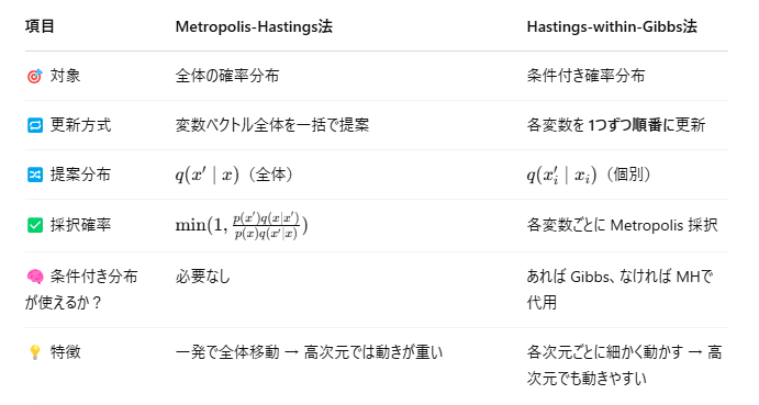
 Metropolis-Hastingsどんな分布に対しても使えるが高次元だと効率が悪い。

⇒ Gibbsサンプリングで1変数ずつ更新する

 Gibbsサンプリング多変量分布から、1変数ずつ直接サンプリングする方法

⇒ 直接サンプリングできない場合がある（条件付き分布を明示的にサンプリングできない

⇒ Hasting-within-Gibbs法


 Hastings-within-GibbsMatropolis-Hastings法は全体の変数を一気に更新するのに対し、Hasting-within-Gibbs法は変数を1つずつ更新し、それぞれにMatropolis-Hastings法を使うという手法である。
条件付き分布はわかるが直接サンプリングできない場合に効果的である。


 Hastings-within-GibbsをPythonで実装してみるimport numpy as np
import matplotlib.pyplot as plt

# 目標分布, 2次元のガウス分布
def target_dist(x, y):
    return np.exp(-0.5 * (x**2 + y**2 + 0.8 * x * y))

# サンプリングの初期設定
num_samples = 5000
samples = np.zeros((num_samples, 2))
x, y = 0.0, 0.0
proposal_std = 0.5 # 提案分布の標準偏差, ジャンプ幅を制御

# Hasting and Gibbs Sampling
for i in range(num_samples):
    # xの更新
    x_prop = np.random.normal(x, proposal_std)
    if np.random.rand() < target_dist(x_prop, y) / target_dist(x, y):
        x = x_prop
        
    # yの更新
    y_prop = np.random.normal(y, proposal_std)
    if np.random.rand() < target_dist(x, y_prop) / target_dist(x, y):
        y = y_prop
        
    samples[i] = [x, y]

# グリッドの生成
x_vals = np.linspace(-3, 3, 200)
y_vals = np.linspace(-3, 3, 200)
X, Y = np.meshgrid(x_vals, y_vals)

# 目標分布の評価
Z = target_dist(X, Y)

# 周辺化のための数値積分を行う
dx = x_vals[1] - x_vals[0]
dy = y_vals[1] - y_vals[0]
marginal_x = Z.sum(axis=0) * dy
marginal_y = Z.sum(axis=1) * dx

# 周辺密度を確率として正規化
area_x = np.trapezoid(marginal_x, x_vals)
area_y = np.trapezoid(marginal_y, y_vals)
marginal_x_norm = marginal_x / area_x
marginal_y_norm = marginal_y / area_y

# スケーリングのために最大値を格納
max_marginal_x = np.max(marginal_x_norm)
max_marginal_y = np.max(marginal_y_norm)

# 3Dプロットの設定
fig = plt.figure(figsize=(8, 8))
ax = fig.add_subplot(111, projection='3d')

# 軸の範囲を設定
ax.set_xlim(X.min(), X.max())
ax.set_ylim(Y.min(), Y.max())
max_pdf = Z.max()
ax.set_zlim(0, max_pdf)

# z=0の平面を描画
Z0 = np.zeros_like(Z)
ax.plot_surface(
    X, Y, Z0,
    alpha=0.0,
    rstride=20, cstride=20,
    edgecolor='none'
)

# サンプルを描画
ax.scatter(
    samples[:, 0], samples[:, 1], np.zeros(num_samples),
    color='red', s=5, alpha=0.4, label='Samples'
)

# 壁の生成
x_min, x_max = ax.get_xlim()
y_min, y_max = ax.get_ylim()

# marginal_x_norm は積分すると1になるように正規化されているが,
# ピークが1を超えている可能性があるので max_marginal_xを使って再度正規化を行う.
# その後, 目標分布の最大値で拡大する.
wall_y = np.full_like(x_vals, y_max)
ax.plot(
    x_vals, wall_y, marginal_x_norm / max_marginal_x * max_pdf,
    color='blue', lw=2, label='p(x) (normalized)'
)

# ここも上と同様に正規化を行う.
wall_x = np.full_like(y_vals, x_min)
ax.plot(
    wall_x, y_vals, marginal_y_norm / max_marginal_y * max_pdf,
    color='green', lw=2, label='p(y) (normalized)'
)

# 軸のラベルとタイトルを設定
ax.set_xlabel("x")
ax.set_ylabel("y")
ax.set_zlabel("Density")
ax.set_title("Hesting and Gibbs Sampling")
ax.legend(loc='upper left')

plt.tight_layout()
plt.show()
MCMCの流れ Metropolis-Hastings法

Pythonで実装してみる

全体のコード

アニメーション版

Metropolis-Hastings

Gibbsサンプリング

Hastings-within-Gibbs

Hastings-within-GibbsをPythonで実装してみる

Discussion
