
この記事は、🎄Explaza Advent Calendar 2025🎄 の8日目の記事です。
はじめに
OpenAI Agents SDK(Responses API)で使えるツールの一つに、CodeInterpreterToolがあります。LLMにPythonコードを生成させて、そのコードをサンドボックス環境で実行できるという機能です。
ChatGPT Webでもコード生成&実行の機能は使えますが、自前のシステムに組み込むことを想定した検証をしたかったので、APIから利用できるCodeInterpreterToolを使って色々試してみました。
今回は「どんなことができそうか」「使い勝手はどうか」をざっくり検証した内容をまとめます。そこまで深追いはしていない、ライトな検証記録です。
CodeInterpreterToolとは
CodeInterpreterToolは、LLMにPythonコードを書かせて、そのコードを実行させることができるツールです。コード実行環境はコンテナでサンドボックス化されており、安全に処理を行うことができます。
基本的な使い方
CodeInterpreterToolを使う流れは以下のようになります。
-
(外部からファイルを与える場合)ファイルをアップロード
処理対象のファイルをOpenAI Files APIでアップロードしておく -
コンテナを作成
アップロードしたファイルのfile_idを指定して、そのファイルをマウントしたコンテナを作成する -
LLMをコール
CodeInterpreterToolのconfigでコンテナのIDを指定し、toolsにCodeInterpreterToolを設定してLLMをコールする -
(必要に応じて)生成ファイルを取得
CodeInterpreterToolが実行した結果として生成されたファイルを取得したい場合は、Container Files APIを使う-
List container files でファイル一覧を取得(LLMのレスポンス内にも
file_idの記載があるのでそちらからID取得してもよい) -
Retrieve container file content で
file_idを指定してファイルの内容を取得
-
List container files でファイル一覧を取得(LLMのレスポンス内にも
コンテナ作成とLLMコールに該当する箇所を実行するサンプルコードは以下のようなイメージです。
import os

from openai import OpenAI
from agents import Agent, Runner, CodeInterpreterTool
from openai.types.responses.tool_param import CodeInterpreter

client = OpenAI()

# 事前にファイルアップロードして発行されたfile_id
# アップロード処理はここでは割愛
file_ids = ["file-xxxxxxxxxxxxxxxxxxxxxx", "file-yyyyyyyyyyyyyyyyyyyyyy"]

# コンテナを作成(ファイルをマウント)
container = client.containers.create(
    name="test-container",
    memory_limit="16g",  # 指定なしの場合デフォルトで "1g"
    file_ids=file_ids
)
container_id = container.id

# CodeInterpreterToolの設定
code_interpreter_tool = CodeInterpreterTool(
    tool_config=CodeInterpreter(
        type="code_interpreter",
        container=container_id,
    )
)

# Agentの作成
agent = Agent(
    name="CodeInterpreterAgent",
    instructions=(
        "You are a helpful assistant that uses the Code Interpreter tool "
        "to analyze the provided files and answer questions about them."
    ),
    model="gpt-5-mini",
    tools=[code_interpreter_tool],
)

# 実行
prompt = "(なにかしらのプロンプト)"
result = Runner.run_sync(
    agent,
    prompt,
)

print(result.final_output)
やってみた:できたこと
データファイルを食わせて分析処理
CodeInterpreterToolといえばデータ分析、という印象があったので、まずはシンプルにCSVファイルを読み込ませて分析させてみました。
基本的な分析向けのパッケージ(pandas、numpy等)がプリインストールされているので、「このCSVを分析して」といった雑な指示でも、それなりに動いてくれます。
今回はKaggleで入手できるSpotifyデータセット(約116万行)をアップロードして、以下のようなプロンプトで処理させてみました。
入力したプロンプト:
あなたはデータ可視化が得意なアナリストです。
アップロードされたCSVについて、どのような可視化が可能か提案し、コードを生成して実行してください。
可視化した画像はファイルとして出力してください(/mnt/data/の下にディレクトリを作らず直接ファイルを置いて下さい)
データ概要と可視化画像を出力したというレスポンスが返ってきました。長くなるのでアコーディオンにしておきます。
レスポンステキストと生成された画像ファイル
レスポンステキスト
ありがとうございます。CSVを読み込み、どの可視化が有益かを提案したうえでいくつかの図を作成・保存しました。作成したファイルはすべて /mnt/data に直接出力しています(ディレクトリは作成していません)。
まずデータ概要(自動検出)
- 行数: 1,159,764
- 列数: 20
- 主な列:
- artist_name, track_name, track_id, popularity, year, genre
- オーディオ特徴: danceability, energy, key, loudness, mode, speechiness, acousticness, instrumentalness, liveness, valence, tempo, duration_ms, time_signature
- 欠損: ほとんどの主要列は欠損なし(今回のファイルはフルに揃っています)
実行前に提案した可視化(代表例)
1. 人気度(popularity)の分布(ヒストグラム) — 人気曲の分布把握
2. 複数のオーディオ特徴の分布(一括表示) — danceability, energy, valence などのばらつき確認
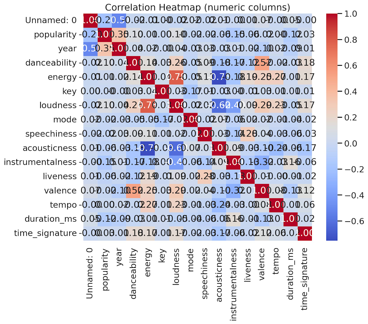
3. 数値カラム同士の相関ヒートマップ — どの特徴が相関しているか
4. tempo vs energy の散布図(人気度で色分け) — 曲のテンポとエネルギーの関係
5. アーティスト別集計(トラック数上位、平均人気度上位) — データ内の主要アーティスト把握
6. (可能なら)リリース年ごとのトレンド(年別の平均人気度や曲数) — 年代変化の把握
今回実際に作成した図(ファイルと簡単な説明)
- spotify_popularity_histogram.png — popularity の分布(ヒストグラム + KDE)
- spotify_audio_features_distributions.png — オーディオ特徴のヒストグラムを複数パネルで表示
- spotify_numeric_correlation_heatmap.png — 数値カラム間の相関係数ヒートマップ
- spotify_tempo_vs_energy_scatter.png — tempo vs energy の散布図(popularity で色分け)
- spotify_top20_artists_by_count.png — トラック数が多いアーティスト上位20
- spotify_top20_artists_by_avg_popularity.png — 平均 popularity が高いアーティスト上位20
(上記のファイルはすべて /mnt/data に配置済みです)
補足・注意点
- データサイズが大きいため(約116万行)、対話的な可視化やペアプロット全列描画は処理負荷が高くなる可能性があります。サンプリングを使うか、列を絞ることを推奨します。
生成された画像ファイル
生成された画像ファイルは下記です。まだ調整の余地がある感じの図になっています。


また、APIのレスポンスからは実際に実行されたコードも抽出できます。参考のためにアコーディオンで添付しておきます。
実行されたコード
# Read the uploaded CSV and inspect its structure, then create a set of informative visualizations.
# The generated image files will be saved directly under /mnt/data as requested.
# We'll first load the file and display a brief summary, then create plots based on available columns.

import pandas as pd
import matplotlib.pyplot as plt
import seaborn as sns
import numpy as np
import os

file_path = "/mnt/data/file-XTcznHy3fzfT513N3kkVKb-spotify_data.csv"
df = pd.read_csv(file_path, low_memory=False)

# Display basic info
info = {
    "rows": df.shape[0],
    "columns": df.shape[1],
    "columns_list": df.columns.tolist(),
    "dtypes": df.dtypes.apply(lambda x: x.name).to_dict(),
    "missing_per_column": df.isna().sum().to_dict()
}

info_summary = pd.DataFrame({
    "column": df.columns,
    "dtype": [str(x) for x in df.dtypes],
    "missing": df.isna().sum().values,
    "unique_values": [df[col].nunique(dropna=True) for col in df.columns]
})

# Print top rows and info summary
print("Data shape:", df.shape)
print("\nFirst 5 rows:")
display(df.head())

print("\nColumn summary:")
display(info_summary)

# Determine numeric audio feature columns commonly found in Spotify datasets
possible_audio_features = ["danceability","energy","key","loudness","mode","speechiness","acousticness",
                           "instrumentalness","liveness","valence","tempo","duration_ms","time_signature","popularity"]

numeric_cols = [c for c in df.columns if pd.api.types.is_numeric_dtype(df[c])]
audio_features = [c for c in possible_audio_features if c in df.columns and c in numeric_cols]

print("\nDetected numeric columns:", numeric_cols)
print("Detected audio/feature columns:", audio_features)

# Create output plots depending on available columns
output_files = []

sns.set(style="whitegrid", context="talk")

# 1) Histogram of popularity (if present)
if "popularity" in df.columns:
    plt.figure(figsize=(8,5))
    sns.histplot(df["popularity"].dropna(), bins=30, kde=True, color="teal")
    plt.title("Distribution of Track Popularity")
    plt.xlabel("Popularity")
    plt.ylabel("Count")
    out1 = "/mnt/data/spotify_popularity_histogram.png"
    plt.savefig(out1, bbox_inches="tight", dpi=150)
    output_files.append(out1)
    plt.close()

# 2) Distribution of audio features (multi-panel)
if len(audio_features) > 0:
    # choose up to 9 features to plot
    features_to_plot = audio_features[:9]
    n = len(features_to_plot)
    cols = 3
    rows = int(np.ceil(n/cols))
    plt.figure(figsize=(5*cols,4*rows))
    for i, feat in enumerate(features_to_plot, start=1):
        plt.subplot(rows, cols, i)
        sns.histplot(df[feat].dropna(), bins=30, kde=True, color="purple")
        plt.title(feat)
    plt.suptitle("Distributions of Audio Features", fontsize=18, y=1.02)
    out2 = "/mnt/data/spotify_audio_features_distributions.png"
    plt.savefig(out2, bbox_inches="tight", dpi=150)
    output_files.append(out2)
    plt.close()

# 3) Correlation heatmap for numeric columns (subset if too many)
if len(numeric_cols) >= 2:
    num_for_corr = df[numeric_cols].select_dtypes(include=[np.number]).corr()
    # limit to 20 columns for readability
    if num_for_corr.shape[1] > 20:
        num_for_corr = num_for_corr.iloc[:20, :20]
    plt.figure(figsize=(10,8))
    sns.heatmap(num_for_corr, annot=True, fmt=".2f", cmap="coolwarm", square=False)
    plt.title("Correlation Heatmap (numeric columns)")
    out3 = "/mnt/data/spotify_numeric_correlation_heatmap.png"
    plt.savefig(out3, bbox_inches="tight", dpi=150)
    output_files.append(out3)
    plt.close()

# 4) Scatter: tempo vs energy (color by popularity if available)
if "tempo" in df.columns and "energy" in df.columns:
    plt.figure(figsize=(8,6))
    if "popularity" in df.columns:
        sc = plt.scatter(df["tempo"], df["energy"], c=df["popularity"], cmap="viridis", alpha=0.7)
        plt.colorbar(sc, label="popularity")
    else:
        plt.scatter(df["tempo"], df["energy"], alpha=0.6)
    plt.xlabel("Tempo")
    plt.ylabel("Energy")
    plt.title("Tempo vs Energy (colored by popularity)" if "popularity" in df.columns else "Tempo vs Energy")
    out4 = "/mnt/data/spotify_tempo_vs_energy_scatter.png"
    plt.savefig(out4, bbox_inches="tight", dpi=150)
    output_files.append(out4)
    plt.close()

# 5) Top artists by track count or by average popularity
if "artist_name" in df.columns or "artists" in df.columns:
    artist_col = "artist_name" if "artist_name" in df.columns else "artists"
    # If artists is a list-like string, try to extract first artist
    artists = df[artist_col].fillna("Unknown").astype(str).apply(lambda x: x.split(";")[0].split(",")[0])
    top_counts = artists.value_counts().head(20)
    plt.figure(figsize=(10,6))
    sns.barplot(y=top_counts.index, x=top_counts.values, palette="magma")
    plt.xlabel("Number of Tracks in Dataset")
    plt.ylabel("Artist")
    plt.title("Top 20 Artists by Track Count")
    out5 = "/mnt/data/spotify_top20_artists_by_count.png"
    plt.savefig(out5, bbox_inches="tight", dpi=150)
    output_files.append(out5)
    plt.close()

    # Average popularity per artist (if popularity exists)
    if "popularity" in df.columns:
        avg_pop = df.assign(artist_first=artists).groupby("artist_first")["popularity"].mean().sort_values(ascending=False).head(20)
        plt.figure(figsize=(10,6))
        sns.barplot(x=avg_pop.values, y=avg_pop.index, palette="viridis")
        plt.xlabel("Average Popularity")
        plt.ylabel("Artist")
        plt.title("Top 20 Artists by Average Popularity")
        out6 = "/mnt/data/spotify_top20_artists_by_avg_popularity.png"
        plt.savefig(out6, bbox_inches="tight", dpi=150)
        output_files.append(out6)
        plt.close()

# 6) Release year trend if release_date exists
date_col = None
for c in df.columns:
    if "release" in c.lower() or "date" in c.lower():
        date_col = c
        break

if date_col is not None:
    # try to parse to datetime
    try:
        dates = pd.to_datetime(df[date_col], errors="coerce")
        df["release_year"] = dates.dt.year
        year_counts = df.dropna(subset=["release_year"]).groupby("release_year").agg({
            "popularity": "mean",
            df.columns[0]: "count"  # just count rows
        }).rename(columns={df.columns[0]: "track_count"})
        if not year_counts.empty:
            plt.figure(figsize=(10,5))
            if "popularity" in df.columns:
                ax = year_counts["popularity"].plot(kind="line", marker="o", color="blue", label="Avg Popularity")
                ax.set_ylabel("Average Popularity")
                ax.set_xlabel("Release Year")
                ax.set_title("Average Popularity by Release Year")
                out7 = "/mnt/data/spotify_avg_popularity_by_year.png"
                plt.savefig(out7, bbox_inches="tight", dpi=150)
                output_files.append(out7)
                plt.close()
            # plot track counts as bar
            plt.figure(figsize=(10,5))
            year_counts["track_count"].plot(kind="bar", color="gray")
            plt.ylabel("Track Count in Dataset")
            plt.xlabel("Release Year")
            plt.title("Track Count by Release Year")
            out8 = "/mnt/data/spotify_track_count_by_year.png"
            plt.savefig(out8, bbox_inches="tight", dpi=150)
            output_files.append(out8)
            plt.close()
    except Exception as e:
        print("Could not parse release dates:", e)

# Summarize generated files
print("\nGenerated the following visualization files:")
for f in output_files:
    print(f)

# Return info dict and list of generated files
info, output_files
フワっとした指示でここまでやってくれるのが面白いと思いつつ、レスポンスが返ってくるまでに結構な所要時間(モデルのreasoning性能にも影響するでしょうが、5〜10分ぐらいかかっていました)がかかったのと、後述する制約を考えると、ガッツリとした分析用途で使うには厳しい印象です。ちょっとしたデータの確認や、軽い集計処理には便利だと思います。あとは出力された画像が気に入らなかったときにどの程度調整などできるのかも気になるところですが、今回はそこまで踏み込みませんでした。
緯度経度データを食わせて地図上にプロット
緯度経度の位置情報を含むデータを渡して「地図上にプロットして」と指示してみました。
渡したデータファイル
id,name,latitude,longitude,based_on_category
1,Tokyo Station,35.681236,139.767125,A
2,Shinjuku,35.689487,139.691706,B
3,Shibuya,35.658034,139.701636,C
4,Ueno,35.713768,139.777254,A
5,Ikebukuro,35.728926,139.710038,B
6,Yokohama,35.465833,139.622222,C
7,Kawasaki,35.530811,139.696972,A
8,Chiba,35.607287,140.106361,B
9,Omiya,35.906908,139.623844,C
10,Funabashi,35.694003,139.982552,A
11,Machida,35.540163,139.450636,B
12,Hachioji,35.655018,139.338955,C
最初は雑な指示だとうまくいかなかったのですが、プリインストールされているパッケージ(foliumなど)を具体的に指定することで、地図上へのプロットができました。
うまくいかなかったプロンプト:
地図描画パッケージを使って、CSVに記載されているポイントを地図に合わせて プロットする画像を作成してください。
このプロンプトだと、期待した出力が得られませんでした。
うまくいったプロンプト:
アップロードしたCSVファイルを使って、緯度経度を地図上にプロットする処理を行ってください。
以下の要件でPythonコードを書いて実行してください。
必要なライブラリ(pandas, geopandas, folium, shapely など)をインポートし、使用バージョンをprintしてください。
CSVファイルを pandas の DataFrame として読み込み、先頭数行とカラム一覧を表示してください。
次のカラムを使って処理してください(必要に応じてコード側でカラム名を調整してください):
緯度カラム名: latitude
経度カラム名: longitude
カテゴリカラム名: based_on_category
ポップアップ用の名称カラム名: name
latitude と longitude から Point ジオメトリを作成し、geopandas の GeoDataFrame に変換してください。
全データの中心付近(緯度・経度の平均)を計算し、その位置を folium マップの初期中心として使ってください。
based_on_category ごとに色を変えてマーカーをプロットしてください。
カテゴリごとに色を割り当てる辞書を定義し、未知のカテゴリがあればデフォルト色を使ってください。
マーカーのポップアップまたはツールチップに name を表示してください。
作成したマップを locations_map.html というファイル名で保存し、そのファイルをダウンロードできるようにしてください。
最後に、処理の手順と、今回使用した主なライブラリの役割を簡単に日本語で説明してください。
途中経過(DataFrameのhead、GeoDataFrameの情報、色分けのマッピングなど)も print して確認できるようにお願いします。
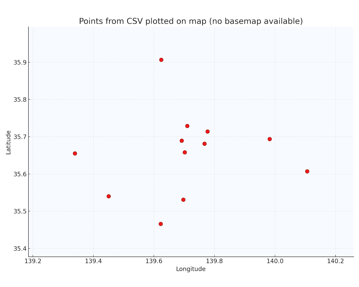
このように具体的な指示を与えることで、Foliumを使ってブラウザで確認できるインタラクティブな地図(HTML形式)が生成されました。下記はブラウザで表示した画像のスクリーンショットです。

プロンプトで使用するパッケージやカラム名を具体的に指定すると、期待通りに動いてくれる感じです。
やってみた:できなかったこと
インターネット上のページにアクセスして内容取得
「このURLにアクセスして内容を取得して」といった処理はできませんでした。
CodeInterpreterToolの実行環境はインターネットに接続できない仕様になっています。セキュリティ上の理由だと思いますが、Web APIを叩いたりスクレイピングしたりといった処理はCodeInterpreterTool単体では不可能です。
(WebSearchToolなど他のツールと組み合わせて得られたコンテキストを流すなどはできそうな気がしますが、今回は検証していません)
任意のPythonパッケージをインストールして使用する
pip installで好きなパッケージを追加することもできません。
インターネットに繋がらないので、PyPIからパッケージを取得することができないためです。プリインストールされているパッケージの範囲内でやりくりする必要があります。
参考のために、CodeInterpreterToolのコンテナにプリインストールされているパッケージの一覧を貼っておきます。(2025年12月8日時点)
プリインストールパッケージ一覧
name,version
absl-py,2.3.1
ace-tools,0.0.1
aeppl,0.0.31
aesara,2.7.3
affine,2.4.0
aiohttp,3.9.5
aiosignal,1.4.0
analytics-python,1.4.post1
annotated-types,0.7.0
anyio,4.9.0
anytree,2.8.0
argon2-cffi,25.1.0
argon2-cffi-bindings,21.2.0
arrow,1.3.0
arviz,0.21.0
asn1crypto,1.5.1
asttokens,3.0.0
async-lru,2.0.5
attrs,25.3.0
audioread,3.0.1
babel,2.17.0
backoff,1.10.0
basemap,1.3.9
basemap-data,1.3.2
bcrypt,4.3.0
beautifulsoup4,4.13.4
bleach,6.2.0
blinker,1.9.0
blis,0.7.11
blosc2,2.0.0
bokeh,2.4.0
branca,0.8.1
Brotli,1.1.0
bytecode,0.16.2
cachetools,6.1.0
cairocffi,1.7.1
CairoSVG,2.5.2
camelot-py,0.10.1
catalogue,2.0.10
catboost,1.2.8
cattrs,24.1.3
certifi,2021.1.10.2
cffi,1.17.1
chardet,3.0.4
charset-normalizer,2.1.1
click,8.2.1
click-plugins,1.1.1.2
cligj,0.7.2
cloudpickle,3.1.1
cmudict,1.1.0
comm,0.2.2
confection,0.1.5
cons,0.4.7
contourpy,1.3.2
countryinfo,0.1.2
coverage,7.5.4
cryptography,3.4.8
cssselect2,0.8.0
cycler,0.12.1
cymem,2.0.11
Cython,0.29.36
databricks-sql-connector,0.9.1
datadog,0.49.1
ddsketch,3.0.1
ddtrace,2.8.7
debugpy,1.8.15
decorator,4.4.2
defusedxml,0.7.1
dlib,19.24.2
dnspython,2.7.0
docx2txt,0.8
einops,0.3.2
email_validator,2.2.0
envier,0.6.1
et_xmlfile,2.0.0
etuples,0.3.10
exchange-calendars,3.4
executing,2.2.0
Faker,8.13.2
fastapi,0.111.0
fastapi-cli,0.0.8
fastjsonschema,2.21.1
fastprogress,1.0.3
ffmpeg-python,0.2.0
ffmpy,0.6.1
filelock,3.18.0
Fiona,1.9.2
Flask,3.1.1
Flask-CacheBuster,1.0.0
flask-cors,6.0.1
Flask-Login,0.6.3
folium,0.12.1
fonttools,4.59.0
fpdf2,2.8.3
fqdn,1.5.1
frozenlist,1.7.0
fsspec,2025.7.0
future,1.0.0
fuzzywuzzy,0.18.0
gensim,4.3.1
geographiclib,1.52
geopandas,0.10.2
geopy,2.2.0
gradio,2.2.15
graphviz,0.17
gTTS,2.2.3
h11,0.16.0
h2,4.2.0
h5netcdf,1.6.3
h5py,3.8.0
hpack,4.1.0
html5lib,1.1
httpcore,1.0.9
httptools,0.6.4
httpx,0.28.1
hypercorn,0.14.3
hyperframe,6.1.0
idna,3.10
imageio,2.37.0
imageio-ffmpeg,0.6.0
imbalanced-learn,0.12.4
imblearn,0.0
imgkit,1.2.2
importlib_metadata,8.7.0
importlib_resources,6.5.2
iniconfig,2.1.0
ipykernel,6.30.0
ipython,9.4.0
ipython-genutils,0.2.0
ipython_pygments_lexers,1.1.1
isodate,0.7.2
isoduration,20.11.0
itsdangerous,2.2.0
jax,0.2.28
jedi,0.19.2
Jinja2,3.1.6
joblib,1.5.1
json5,0.12.0
jsonpickle,4.1.1
jsonpointer,3.0.0
jsonschema,4.25.0
jsonschema-specifications,2025.4.1
jupyter_client,8.6.1
jupyter_core,5.5.1
jupyter-events,0.12.0
jupyter-lsp,2.2.6
jupyter_server,2.14.0
jupyter_server_terminals,0.5.3
jupyterlab,4.1.8
jupyterlab_pygments,0.3.0
jupyterlab_server,2.27.1
keras,2.6.0
kerykeion,2.1.16
kiwisolver,1.4.8
korean-lunar-calendar,0.3.1
langcodes,3.5.0
language_data,1.3.0
lark,1.2.2
lazy_loader,0.4
librosa,0.8.1
lightgbm,4.5.0
llvmlite,0.44.0
logical-unification,0.4.3
loguru,0.5.3
lxml,6.0.0
marisa-trie,1.2.1
markdown-it-py,3.0.0
markdown2,2.5.3
markdownify,0.9.3
MarkupSafe,3.0.2
matplotlib,3.6.3
matplotlib-inline,0.1.7
matplotlib-venn,0.11.6
mdurl,0.1.2
miniKanren,1.0.5
mistune,3.1.3
mizani,0.10.0
mne,0.23.4
monotonic,1.6
moviepy,1.0.3
mpmath,1.3.0
msgpack,1.1.1
mtcnn,0.1.1
multidict,6.6.3
multipledispatch,1.0.0
munch,4.0.0
murmurhash,1.0.13
mutagen,1.45.1
nashpy,0.0.35
nbclassic,0.4.5
nbclient,0.10.2
nbconvert,7.16.6
nbformat,5.10.4
nest-asyncio,1.6.0
networkx,2.8.8
nltk,3.9.1
notebook,6.5.1
notebook_shim,0.2.4
numba,0.61.2
numexpr,2.11.0
numpy,1.24.0
numpy-financial,1.0.0
odfpy,1.4.1
opencv-python,4.5.5.62
openpyxl,3.0.10
opentelemetry-api,1.35.0
opt_einsum,3.4.0
orjson,3.11.0
oscrypto,1.3.0
overrides,7.7.0
packaging,25.0
pandas,1.5.3
pandocfilters,1.5.1
paramiko,3.5.1
parso,0.8.4
pathlib_abc,0.1.1
pathy,0.11.0
patsy,1.0.1
pdf2image,1.16.3
pdfkit,0.6.1
pdfminer.six,20220319
pdfplumber,0.6.2
pdfrw,0.4
pexpect,4.9.0
Pillow,9.1.0
pip,24.0
platformdirs,4.3.8
plotly,5.3.0
plotnine,0.10.1
pluggy,1.6.0
pooch,1.8.2
preshed,3.0.10
priority,2.0.0
proglog,0.1.12
prometheus_client,0.22.1
prompt_toolkit,3.0.51
pronouncing,0.2.0
propcache,0.3.2
protobuf,6.31.1
psutil,7.0.0
ptyprocess,0.7.0
pure_eval,0.2.3
py-cpuinfo,9.0.0
pycountry,20.7.3
pycparser,2.22
pycryptodome,3.23.0
pycryptodomex,3.23.0
pydantic,2.9.2
pydantic_core,2.23.4
pydantic-extra-types,2.10.5
pydantic-settings,2.10.1
pydot,1.4.2
pydub,0.25.1
pydyf,0.11.0
Pygments,2.19.2
pygraphviz,1.7
PyJWT,2.10.1
pylog,1.1
pyluach,2.2.0
pymc,4.0.1
PyMuPDF,1.21.1
PyNaCl,1.5.0
pyOpenSSL,21.0.0
pypandoc,1.6.3
pyparsing,3.2.3
PyPDF2,3.0.1
pyphen,0.17.2
pyproj,3.6.1
pyprover,0.5.6
pyshp,2.3.1
pyswisseph,2.10.3.2
pytesseract,0.3.8
pytest,8.2.2
pytest-asyncio,0.23.8
pytest-cov,5.0.0
pytest-json-report,1.5.0
pytest-metadata,3.1.1
pyth3,0.7
python-dateutil,2.9.0.post0
python-docx,0.8.11
python-dotenv,1.1.1
python-json-logger,2.0.7
python-multipart,0.0.20
python-pptx,0.6.21
pyttsx3,2.90
pytz,2025.2
PyWavelets,1.8.0
pyxlsb,1.0.8
PyYAML,6.0.2
pyzbar,0.1.8
pyzmq,27.0.0
qrcode,7.3
RapidFuzz,3.10.1
rarfile,4.0
rasterio,1.3.3
rdflib,6.0.0
rdkit,2024.9.6
referencing,0.36.2
regex,2024.11.6
reportlab,3.6.12
requests,2.31.0
resampy,0.4.3
rfc3339-validator,0.1.4
rfc3986-validator,0.1.1
rfc3987-syntax,1.1.0
rich,14.0.0
rich-toolkit,0.14.8
rpds-py,0.26.0
scikit-image,0.20.0
scikit-learn,1.1.3
scipy,1.14.1
seaborn,0.11.2
Send2Trash,1.8.3
setuptools,65.5.1
shap,0.39.0
Shapely,1.7.1
shellingham,1.5.4
six,1.17.0
slicer,0.0.7
smart-open,6.4.0
sniffio,1.3.1
snowflake-connector-python,2.7.12
snuggs,1.4.7
SoundFile,0.10.2
soupsieve,2.7
spacy,3.4.4
spacy-legacy,3.0.12
spacy-loggers,1.0.5
sqlparse,0.5.3
srsly,2.5.1
stack-data,0.6.3
starlette,0.37.2
statsmodels,0.13.5
svglib,1.1.0
svgwrite,1.4.1
sympy,1.13.1
tables,3.8.0
tabula,1.0.5
tabulate,0.9.0
tenacity,9.1.2
terminado,0.18.1
text-unidecode,1.3
textblob,0.15.3
thinc,8.1.12
threadpoolctl,3.6.0
thrift,0.22.0
tifffile,2025.6.11
tinycss2,1.4.0
toml,0.10.2
toolz,1.0.0
torch,2.5.1+cpu
torchaudio,2.5.1
torchtext,0.18.0
torchvision,0.20.1
tornado,6.5.1
tqdm,4.64.0
traitlets,5.14.3
trimesh,3.9.29
typer,0.16.0
types-python-dateutil,2.9.0.20250708
typing_extensions,4.14.1
typing-inspection,0.4.1
ujson,5.10.0
uri-template,1.3.0
urllib3,1.26.20
uvicorn,0.19.0
uvloop,0.21.0
Wand,0.6.13
wasabi,0.10.1
watchfiles,1.1.0
wcwidth,0.2.13
weasyprint,53.3
webcolors,24.11.1
webencodings,0.5.1
websocket-client,1.8.0
websockets,10.3
Werkzeug,3.1.3
wheel,0.43.0
wordcloud,1.9.2
wsproto,1.2.0
xarray,2024.3.0
xarray-einstats,0.8.0
xgboost,1.4.2
xlsxwriter,3.2.5
xml-python,0.4.3
xmltodict,0.14.2
yarl,1.20.1
zipp,3.23.0
zopfli,0.2.3.post1
ちなみに、このパッケージ一覧は以下のようなプロンプトでCodeInterpreterToolにコード生成&実行させた結果を観測したものです。
pip listを実行してインストールされているパッケージ一覧を出力してください
なお、OpenAI公式としてはCodeInterpreterToolのコンテナに何のパッケージがプリインストールされているかの仕様は明確にドキュメントにされていません。そのため、前触れなく内容が変わる可能性がある点にはご注意ください。
制約まとめ
検証やドキュメントの確認を通じて把握した制約を整理します。
| 項目 | 内容 |
|---|---|
| ネットワーク | インターネットには接続できない |
| パッケージ | プリインストールされているパッケージのみ使用可能。pip等での追加インストール不可 |
| ファイルサイズ | 1ファイルにつき512MBまで |
| ストレージ上限 | Organization全体で1TBまで |
| メモリ | デフォルト1GB。1GB / 4GB / 16GB / 64GBから選択可能 |
| コンテナ寿命 | 20分で破棄される |
ファイルアップロードについては、それなりに時間がかかる印象でした。180MBのファイルのアップロードに5分強かかりました。ドキュメントではファイルサイズに512MBの制約と書かれているので、ギリギリ制約に引っかからない500MBのファイルでアップロードの実験をしたところ、サイズ上限エラー以前にタイムアウトエラーになりました。サイズの制約にかかるよりも先にタイムアウトの壁に阻まれそうです。
また、コンテナのメモリは指定なしで1GBであり、180MBくらいのファイルを処理させようとしたときに、デフォルトの1GBメモリだと処理ができず、メモリを増やす必要がありました。
コンテナが20分で破棄される制約については、長時間かかる処理の途中でコンテナが消えてエラーになるケースがありました。
ハマりポイント
検証中にハマったポイントをいくつか紹介します。
生成ファイルの保存場所
CodeInterpreterToolで生成されたファイルを取得する際、/mnt/data/ の下に保存されたファイルでないと取得できませんでした。
実際に遭遇した事例を紹介します。先ほどのSpotifyデータの分析を行った際のことです。
最初に試して失敗したプロンプト:
あなたはデータ可視化が得意なアナリストです。
アップロードされたCSVについて、どのような可視化が可能か提案し、コードを生成して実行してください。
可視化した画像はファイルとして出力してください。
このプロンプトで実行すると、LLMが気を利かせて /mnt/data/spotify_visualizations/ というサブディレクトリを作成し、その下に出力ファイルを生成しました。しかし、Container Files APIで取得しようとすると、このサブディレクトリ内のファイルが見えない状態でした。
修正して成功したプロンプト:
あなたはデータ可視化が得意なアナリストです。
アップロードされたCSVについて、どのような可視化が可能か提案し、コードを生成して実行してください。
可視化した画像はファイルとして出力してください(/mnt/data/の下にディレクトリを作らず直接ファイルを置いて下さい)
/mnt/data/ 直下にファイルを配置するよう明示的に指示したところ、Container Files APIから正常に取得できるようになりました。
プロンプトで出力先を明示的に指定しておくと安心です。
日本語フォントの問題
グラフや画像を生成する際に日本語を含めると、フォントの問題で文字化けしてしまうようです。私自身で深く検証できていませんが、覚えておきたいトピックだと思ったので、既に対応方法まで含めて検証されている記事を紹介させていただきます。
この記事では、事前にフォントファイルをアップロードしてコンテナ内にマウントし、そのフォントを使用するようプロンプトで指示する方法が紹介されています。
所感
CodeInterpreterToolは、がっつりとした処理よりも、軽い用途で色々試すのに向いている印象です。
- ちょっとしたデータの確認や可視化
- 簡単な計算処理
- プロトタイプレベルでの検証
といった場面では便利に使えそうです。
一方で、これをプロダクトに組み込んでサービスを作るとなると、制約やアンコントローラブルな部分が多くて難しそうだなという感触でした。特に、コンテナの寿命やメモリ制限、使えるパッケージが保証されていない点などは、本番運用を考えると気になるポイントです。
とはいえ、LLMにコードを書かせて実行させるという体験自体は楽しいものがあります。「こういうことできる?」と試行錯誤する過程で、AI技術の可能性を感じられるツールだと思います。
参考情報
- OpenAI Platform - Agents SDK
- OpenAI Platform - Code Interpreter
- OpenAI API Reference - Container Files

「プロダクトの力で、豊かな暮らしをつくる」をミッションに、法人向けに生成AIのPoC、コンサルティング〜開発を支援する事業を展開しております。 エンジニア募集しています。カジュアル面談応募はこちらから: herp.careers/careers/companies/explaza
Discussion