はじめに
本記事では標準ベイズ統計学の6章で掲載されている図表やモデルをPythonで実装する方法に関して説明します。
6章:ギブスサンプラーによる事後分布の近似
複数のパラメータを持つ統計モデルでは、事後分布の直接的なサンプリングが困難な場合が多いです。しかし、ギブスサンプラーという手法を使えば、この問題を効果的に解決できます。6章ではそのギブスサンプラーに関する説明がされています。
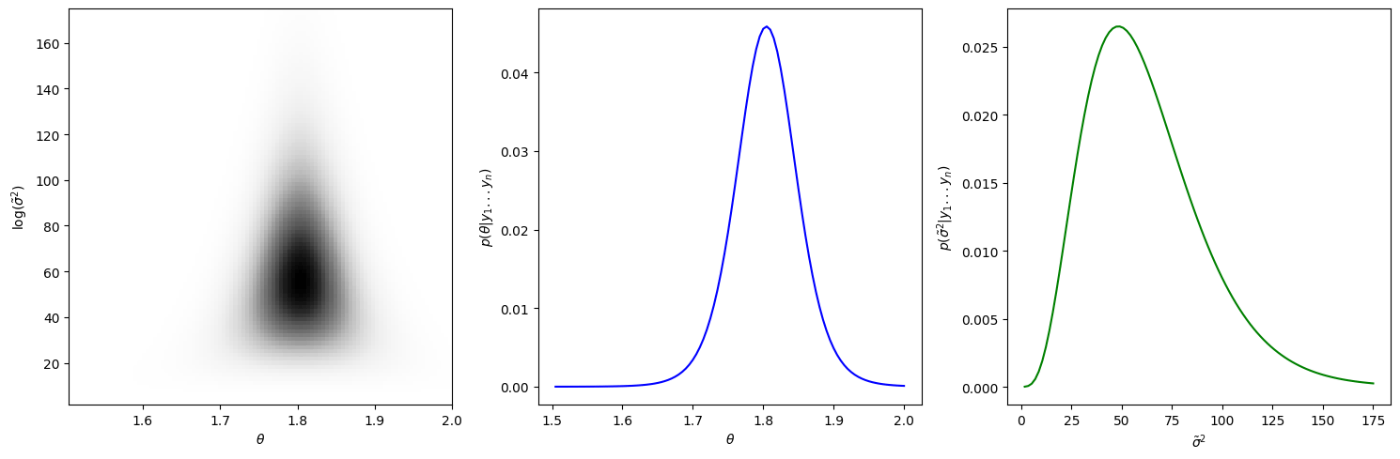
離散近似に基づく同時および周辺事後分布
図6.1では離散近似に基づく同時および周辺事後分布をプロットしています。平均と精度の事後分布を連続的な領域で計算していますが、実際の計算では有限のグリッドを使用しており、そのグリッド上での離散的な近似を行っています。
具体的には、連続的な平均と精度の領域をグリッドに分割し、各グリッドポイントでの事後確率を計算します。このため、得られる事後分布は、実際には連続的な関数ではなく、離散的な値の集合となります。
import numpy as np
from scipy.stats import norm, gamma, gaussian_kde
import matplotlib.pyplot as plt

# データとパラメータの定義
y = np.array([1.64, 1.70, 1.72, 1.74, 1.82, 1.82, 1.82, 1.90, 2.08])
n = len(y)
mean_y = np.mean(y)
var_y = np.var(y)

mu0, t20 = 1.9, 0.95**2
s20, nu0 = 0.01, 1

# 事後分布のグリッドを計算
def calculate_posterior_grid():
    G, H = 100, 100
    mean_grid = np.linspace(1.505, 2.00, G)
    prec_grid = np.linspace(1.75, 175, H)
    post_grid = np.zeros((G, H))

    for g in range(G):
        for h in range(H):
            post_grid[g, h] = (
                norm.pdf(mean_grid[g], mu0, np.sqrt(t20)) *
                gamma.pdf(prec_grid[h], nu0/2, scale=2/(s20*nu0)) *
                np.prod(norm.pdf(y, mean_grid[g], 1/np.sqrt(prec_grid[h])))
            )

    post_grid /= np.sum(post_grid)
    return mean_grid, prec_grid, post_grid

mean_grid, prec_grid, post_grid = calculate_posterior_grid()

# 平均と精度の事後分布の和を計算
mean_post = np.sum(post_grid, axis=1)  # 精度について合計
prec_post = np.sum(post_grid, axis=0)  # 平均について合計

# グリッドをRの出力に合わせて転置(θをy軸、精度をx軸に)
post_grid_transposed = post_grid.T

fig, axs = plt.subplots(1, 3, figsize=(15, 5))

# プロット1: 転置した事後分布のグリッド
axs[0].imshow(post_grid_transposed, extent=[mean_grid.min(), mean_grid.max(), prec_grid.min(), prec_grid.max()],
              origin='lower', cmap='Greys', aspect='auto')
axs[0].set_xlabel(r'$\theta$')
axs[0].set_ylabel(r'log($\tilde{\sigma}^2$)')

# プロット2: 平均(θ)の事後分布
axs[1].plot(mean_grid, mean_post, color='blue')
axs[1].set_xlabel(r'$\theta$')
axs[1].set_ylabel(r'$p(\theta|y_1...y_n)$')

# プロット3: 精度(σ^2)の事後分布
axs[2].plot(prec_grid, prec_post, color='green')
axs[2].set_xlabel(r'$\tilde{\sigma}^2$')
axs[2].set_ylabel(r'$p(\tilde{\sigma}^2|y_1...y_n)$')

plt.tight_layout()
plt.show()
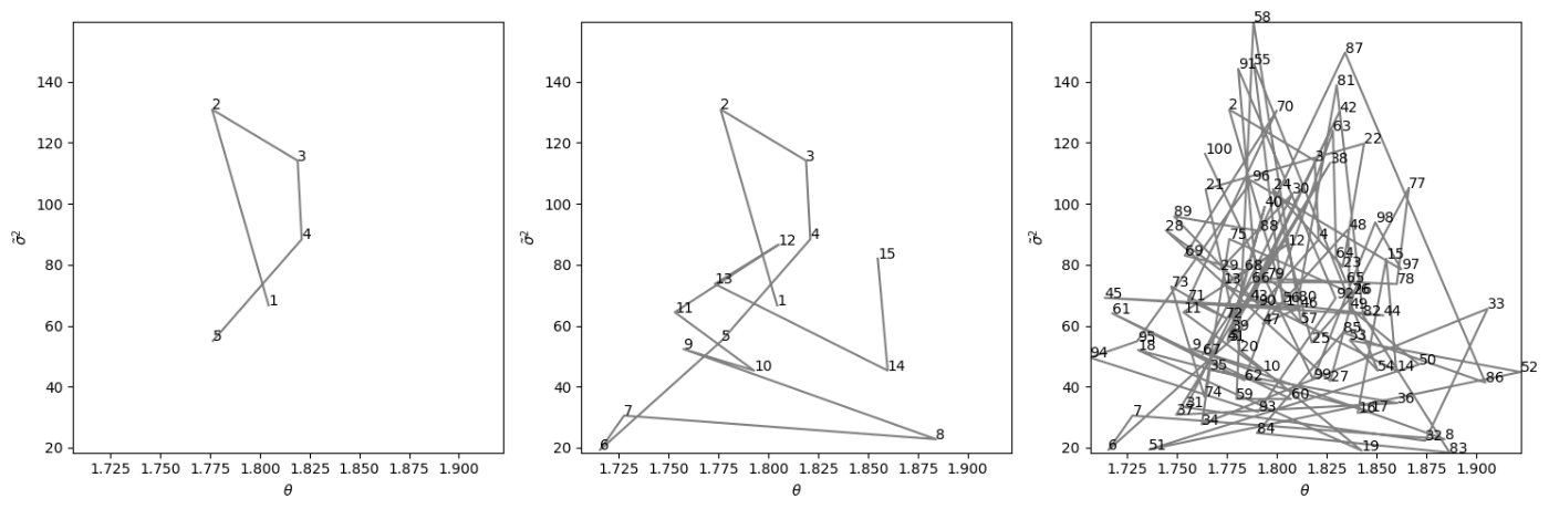
ギブスサンプラーの最初の5回、15回、100回の反復の結果
図6.2はギブスサンプラーの最初の5回、15回、100回の反復の結果です。
ギブスサンプラーのアルゴリズムは以下のとおりです。
この関数はガンマ分布の密度の形をしているため、
となります。
また、
まとめると、
となります。
# 乱数のシードを設定
np.random.seed(30)

# ギブスサンプラー
def gibbs_sampler(S):
    PHI = np.zeros((S, 2))
    PHI[0] = [mean_y, 1/var_y]

    for s in range(1, S):
        mun = (mu0/t20 + n*mean_y*PHI[s-1, 1]) / (1/t20 + n*PHI[s-1, 1])
        t2n = 1 / (1/t20 + n*PHI[s-1, 1])
        PHI[s, 0] = np.random.normal(mun, np.sqrt(t2n))

        nun = nu0 + n
        s2n = (nu0*s20 + (n-1)*var_y + n*(mean_y - PHI[s, 0])**2) / nun
        PHI[s, 1] = np.random.gamma(nun/2, 2/(nun*s2n))

    return PHI

# ギブスサンプラーを実行
S = 1000
PHI = gibbs_sampler(S)

fig, axs = plt.subplots(1, 3, figsize=(15, 5))

m1_values = [5, 15, 100]
for i, m1 in enumerate(m1_values):
    axs[i].plot(PHI[:m1, 0], PHI[:m1, 1], 'gray')
    for j in range(m1):
        axs[i].text(PHI[j, 0], PHI[j, 1], str(j + 1))
    axs[i].set_xlim(PHI[:100, 0].min(), PHI[:100, 0].max())
    axs[i].set_ylim(PHI[:100, 1].min(), PHI[:100, 1].max())
    axs[i].set_xlabel(r'$\theta$')
    axs[i].set_ylabel(r'$\tilde{\sigma}^2$')

plt.tight_layout()
plt.show()
ギブスサンプラーの実装
# ギブスサンプラー
def gibbs_sampler(S):
    PHI = np.zeros((S, 2))
    PHI[0] = [mean_y, 1/var_y]

    for s in range(1, S):
        mun = (mu0/t20 + n*mean_y*PHI[s-1, 1]) / (1/t20 + n*PHI[s-1, 1])
        t2n = 1 / (1/t20 + n*PHI[s-1, 1])
        PHI[s, 0] = np.random.normal(mun, np.sqrt(t2n))

        nun = nu0 + n
        s2n = (nu0*s20 + (n-1)*var_y + n*(mean_y - PHI[s, 0])**2) / nun
        PHI[s, 1] = np.random.gamma(nun/2, 2/(nun*s2n))

    return PHI
ここで、
の実装を行なっています。
初期化
PHI = np.zeros((S, 2))
PHI[0] = [mean_y, 1/var_y]
-
PHIは、各反復でのθとσ^2の値を格納する配列 - 初期値として、データの平均(θの初期値)とデータの精度(σ^2の初期値)を使用
\theta
mun = (mu0/t20 + n*mean_y*PHI[s-1, 1]) / (1/t20 + n*PHI[s-1, 1])
t2n = 1 / (1/t20 + n*PHI[s-1, 1])
PHI[s, 0] = np.random.normal(mun, np.sqrt(t2n))
ここでは
\sigma^2
nun = nu0 + n
s2n = (nu0*s20 + (n-1)*var_y + n*(mean_y - PHI[s, 0])**2) / nun
PHI[s, 1] = np.random.gamma(nun/2, 2/(nun*s2n))
ここでは
上記の過程を繰り返すことで、
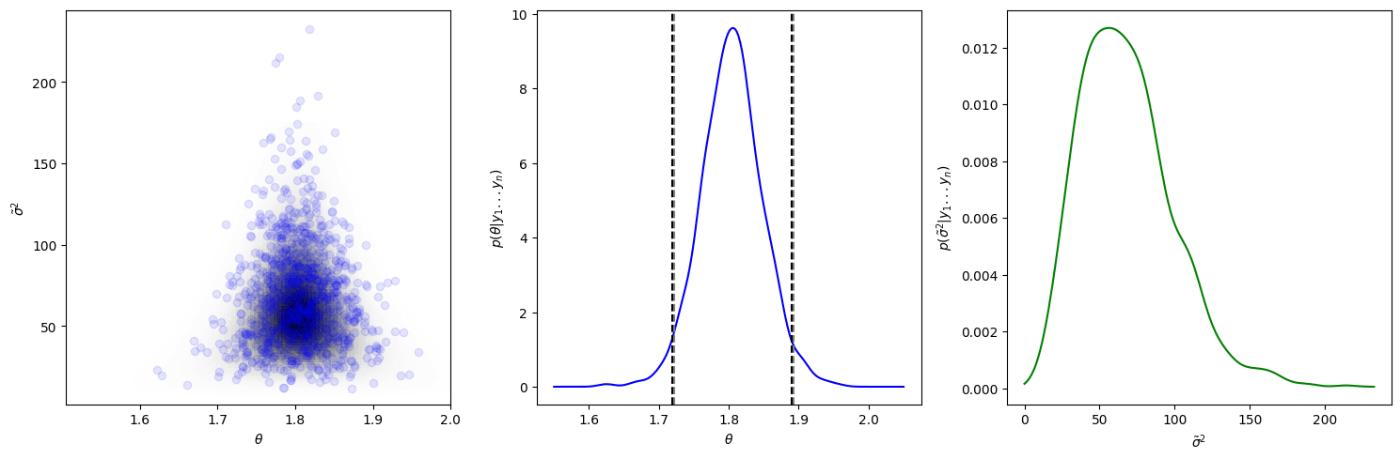
ギブスサンプラーの1000標本と離散近似の等高線、\theta \tilde{\sigma}^2
図6.3では、左図にはギブスサンプラーで得られた1000個の標本を離散近似の等高線とともに表示し、中央と右の図には
# t検定の信頼区間計算
def t_test_confidence_interval(data, confidence=0.95):
    n = len(data)
    mean = np.mean(data)
    se = np.std(data, ddof=1) / np.sqrt(n)
    df = n - 1
    alpha = 1 - confidence
    t_value = np.abs(norm.ppf(alpha/2))
    margin_of_error = t_value * se
    ci_lower = mean - margin_of_error
    ci_upper = mean + margin_of_error
    return ci_lower, ci_upper

fig, axs = plt.subplots(1, 3, figsize=(15, 5))

post_grid_transposed = post_grid.T
axs[0].imshow(post_grid_transposed, extent=[mean_grid.min(), mean_grid.max(), prec_grid.min(), prec_grid.max()],
              origin='lower', cmap='Greys', aspect='auto')
axs[0].scatter(PHI[:, 0], PHI[:, 1], alpha=0.1, c='blue')
axs[0].set_xlabel(r'$\theta$')
axs[0].set_ylabel(r'$\tilde{\sigma}^2$')

theta_density = gaussian_kde(PHI[:, 0])
theta_x = np.linspace(1.55, 2.05, 200)
axs[1].plot(theta_x, theta_density(theta_x), color='blue')

theta_credible_interval = np.percentile(PHI[:, 0], [2.5, 97.5])
axs[1].axvline(x=theta_credible_interval[0], color='gray', linestyle='--')
axs[1].axvline(x=theta_credible_interval[1], color='gray', linestyle='--')

t_conf_int = t_test_confidence_interval(y)
axs[1].axvline(x=t_conf_int[0], color='black', linestyle='--')
axs[1].axvline(x=t_conf_int[1], color='black', linestyle='--')

axs[1].set_xlabel(r'$\theta$')
axs[1].set_ylabel(r'$p(\theta|y_1...y_n)$')

sigma_density = gaussian_kde(PHI[:, 1])
sigma_x = np.linspace(0, np.max(PHI[:, 1]), 200)
axs[2].plot(sigma_x, sigma_density(sigma_x), color='green')
axs[2].set_xlabel(r'$\tilde{\sigma}^2$')
axs[2].set_ylabel(r'$p(\tilde{\sigma}^2|y_1...y_n)$')

plt.tight_layout()
plt.show()
print(f"ベイズ信用区間: {theta_credible_interval}")
print(f"t検定信頼区間: {t_conf_int}")
# ベイズ信用区間: [1.7215529  1.89258362]
# t検定信頼区間: (1.7195685295790368, 1.8893203593098526)
上の図でもわかると思いますが、この結果を見ると、よりt検定による信頼区間とベイズ信用区間がほとんど一致していることがわかると思います。
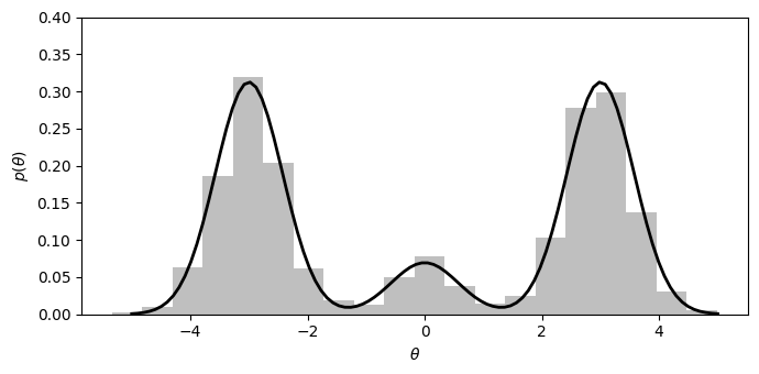
正規密度の混合とモンテカルロ近似
図6.4は以下の三つの正規分布の混合とモンテカルロ近似です。
mu = np.array([-3, 0, 3])
s2 = np.array([0.33, 0.33, 0.33])
w = np.array([0.45, 0.1, 0.45])

ths = np.linspace(-5, 5, 100)
pdf = sum(w[i] * norm.pdf(ths, mu[i], np.sqrt(s2[i])) for i in range(3))

S = 2000
d = np.random.choice(3, size=S, p=w)
th = norm.rvs(mu[d], np.sqrt(s2[d]))

plt.figure(figsize=(7, 3.5))
plt.hist(th, bins=20, density=True, alpha=0.5, color='gray')
plt.plot(ths, pdf, 'k-', linewidth=2)
plt.xlabel(r'$\theta$')
plt.ylabel(r'$p(\theta)$')
plt.ylim(0, 0.40)
plt.tight_layout()
plt.show()
1000,10000個のギブス標本によるヒストグラムとトレースプロット
図6.5、6.6ではギブスサンプリングを用いて混合正規分布からギブス標本を生成し、そのギブス標本のヒストグラムとトレースプロットを表示しています。
図6,5はギブス標本1000個、図6.6は10000個のデータがプロットされています。
def gibbs_sampling_mixture_normal(S):
  np.random.seed(10)
  mu = np.array([-3, 0, 3])
  s2 = np.array([0.33, 0.33, 0.33])
  w = np.array([0.45, 0.1, 0.45])

  th = 0
  THD_MCMC = np.zeros((S, 2))

  for s in range(S):
      p = w * norm.pdf(th, mu, np.sqrt(s2))
      p = p / np.sum(p)
      d = np.random.choice(3, p=p)
      th = norm.rvs(mu[d], np.sqrt(s2[d]))
      THD_MCMC[s] = [th, d]

  fig, (ax1, ax2) = plt.subplots(1, 2, figsize=(14, 3.5))

  ths = np.linspace(-6, 6, 1000)
  pdf = sum(w[i] * norm.pdf(ths, mu[i], np.sqrt(s2[i])) for i in range(3))

  ax1.hist(THD_MCMC[:, 0], bins=20, density=True, alpha=0.5, color='gray')
  ax1.plot(ths, pdf, 'k-', linewidth=2)
  ax1.set_xlabel(r'$\theta$')
  ax1.set_ylabel(r'$p(\theta)$')
  ax1.set_ylim(0, 0.40)

  ax2.scatter(range(S), THD_MCMC[:, 0], alpha=0.5, s=1)
  ax2.set_xlabel('number of iterations')
  ax2.set_ylabel(r'$\theta$')

  plt.tight_layout()
  plt.show()

gibbs_sampling_mixture_normal(1000)
gibbs_sampling_mixture_normal(10000)
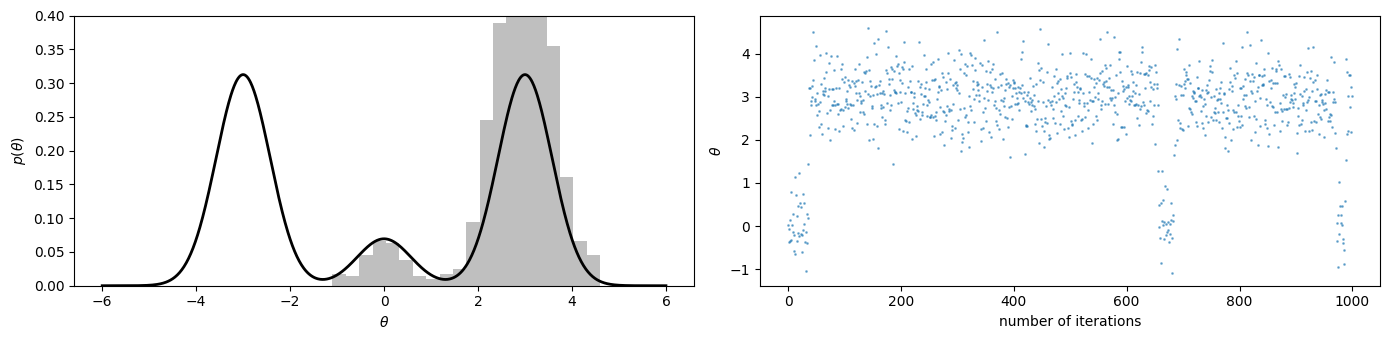
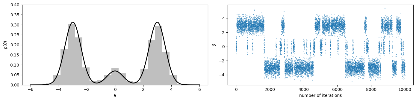
シード値によって分布の形は異なると思いますが、反復回数が増えるにつれて、近似がうまくいっているのがわかると思います。
混合正規分布のギブスサンプリング
for s in range(S):
    p = w * norm.pdf(th, mu, np.sqrt(s2))
    p = p / np.sum(p)
    d = np.random.choice(3, p=p)
    th = norm.rvs(mu[d], np.sqrt(s2[d]))
    THD_MCMC[s] = [th, d]
この部分でギブスサンプリングを用いて混合正規分布からギブス標本を生成しています。
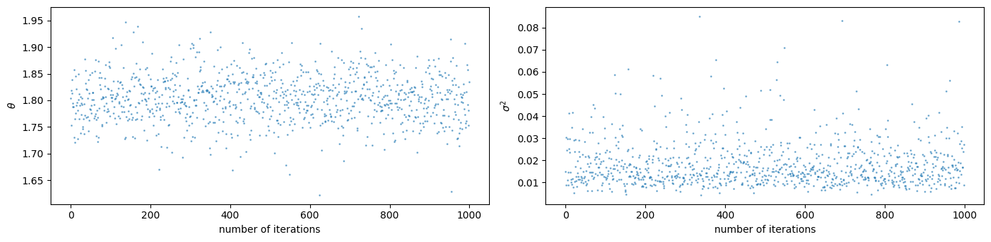
\theta \sigma^2
図6.7は図6.3をプロットする際に行なったギブスサンプラーによって生成された
fig, (ax1, ax2) = plt.subplots(1, 2, figsize=(14, 3.5))

ax1.scatter(range(len(PHI)), PHI[:, 0], alpha=0.5, s=1)
ax1.set_xlabel('number of iterations')
ax1.set_ylabel(r'$\theta$')

ax2.scatter(range(len(PHI)), 1/PHI[:, 1], alpha=0.5, s=1)
ax2.set_xlabel('number of iterations')
ax2.set_ylabel(r'$\sigma^2$')

plt.tight_layout()
plt.show()
最後に
本ブログでは、標準ベイズ統計学の6章で扱われているギブスサンプラーについて、Pythonを用いて実装し、視覚化を行いました。次回は7章「多変量正規モデル」の内容をPythonで実装したいと思います。

Discussion